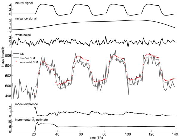
Figure 2.
Example of synthetic fMRI timecourse generation. The top three panels show individual components of the resulting signal. The top panel shows the contribution to the final signal from hemodynamic response to activation (1% signal change). The second panel shows the contribution from scanner drift or physiological noise, measured from real resting fMRI scans (in this case 0.5% signal change). The third panel shows the Gaussian white noise vector generated for this example (SNR of 2). The large panel shows the resulting fMRI timecourse data (the sum of the first three panels and a constant 500 unit offset), the post-hoc GLM reconstruction of this timecourse, and the incremental GLM reconstruction from a fit performed only on data up to that time. Below this, the model difference panel shows the reconstruction error, which is the squared difference between the post-hoc and incremental reconstructions. The bottom panel shows the evolution of the model parameter estimate of the neural basis, which stabilizes near the correct value of 4 after the first stimulus block.

