Figure 5. Shape gives insight into biochemistry.

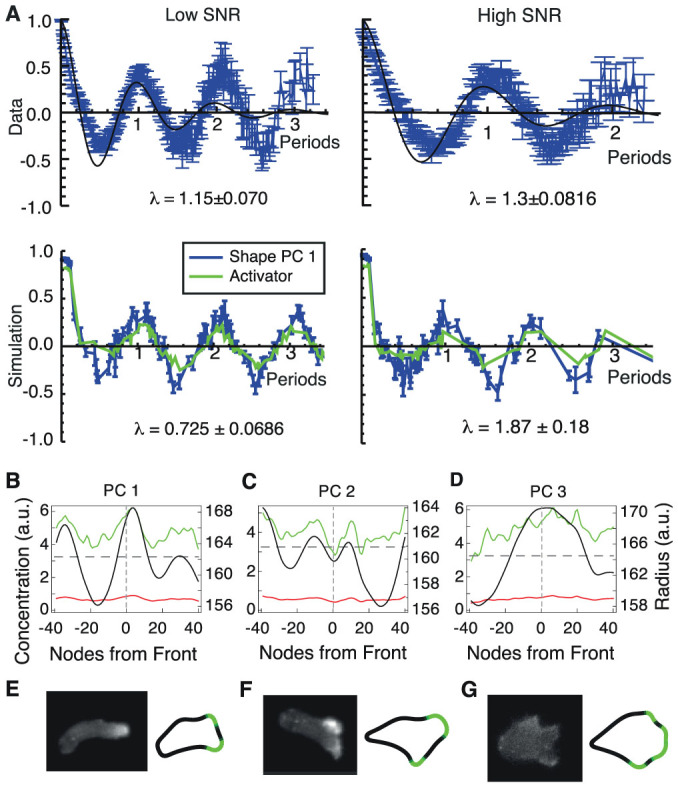
(A) (Top) Average of autocorrelations in PC 1 for live cells, scaled by native period, for 103 low-SNR cells (left) and 78 high-SNR cells (right). The period of each cell's autocorrelation was obtained by selecting the largest mode in the frequency domain. The median periods for low and high SNR were 173.1 s and 239.0 s respectively, reflecting the high persistence of cell shape in high-SNR environments. Simulations captured this trend, with median periods of low- and high-SNR simulations of 126.0 time steps and 240.5 time steps, respectively. Error-bars on autocorrelations are large-lag standard errors. (Bottom) Autocorrelations of PC 1 (blue) and of local activator (green) for simulated shallow (left) and steep (right) gradient cells. Individual autocorrelations are aligned according to their fundamental periods, and then averaged. Similar to live cell data, the simulated cells have oscillatory autocorrelations in PC 1, which are less apparent in the steep gradient. For live cell autocorrelations in other PCs, see Fig. S6. (B–D). Concentrations of activator (green), local inhibitor (red) and global inhibitor (dark grey, dashed) and radii (black) are averaged over cells with high values of PC 1 (B), PC 2 (C) and PC 3 (D) and plotted as functions of nodes around the cell contour. Concentration values are shown on the left axis and radii on the right axis. Plots are aligned with the direction of motion in the centre and the rear of the cell at the far left and right. (E–G) Examples of live cells with limGFP-labeled actin (left) compared with simulated cell shapes (right). Cells and simulations in (E) and (F) are exposed to a low SNR. The cell and simulation in (G) are exposed to a high SNR.