Fig. 1.

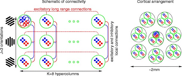
Left: Schematic diagram of network architecture. Our network comprises a 2D array of ‘clusters’ (green circles) each containing a few hundred excitatory (red) and inhibitory (blue) neurons. Rows correspond to clusters with the same orientation preference and columns represent hypercolums. We refer to C _jk as the jth orientation domain in the kth hypercolumn. Neurons within each cluster are connected via local excitatory and inhibitory connections (as indicated by red and blue lines within one representative cluster). Clusters with different orientation preferences within a hypercolumn (i.e., C _1k, C _2k, …) are also connected via local connections. Clusters of the same orientation preference in different hypercolumns (i.e,. C _j1, C _j2, …) are connected via excitatory long-range connections (as indicated by dashed red lines). Local connectivity both within each cluster and between clusters in the same hypercolumn is statistically homogeneous; neurons are sparsely and randomly connected to one another, with slightly higher connectivity among neurons within a cluster. Long-range connectivity between clusters with like orientation-preference in different hypercolumns is also statistically homogeneous. For simulations we use a network with 3 orientation domains in each of 8 hypercolumns. Right: Hypercolumn arrangement. Eight hypercolumns, each containing 3 clusters corresponding to distinct orientation domains, are depicted by dashed circles; all pairs of hypercolumns are thought of as ‘adjacent’, or ‘equal distance’ apart. Our network is intended to model a ∼ 2 mm² patch of cortex: large enough to contain several hypercolumns, but small enough that the long-range connectivities between any two pairs of hypercolumns are roughly similar