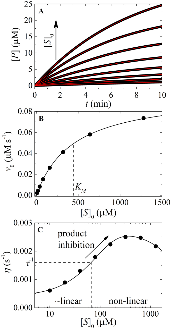
Figure 2. Analysis of non-linear enzyme kinetic time courses.

(A). Simulated enzyme cycling time courses according to Figure A1 with initial [substrate] (from bottom to top) of 10, 20, 40, 80, 160, 320, 640, and 1280 μM, and the following fundamental reaction rate constants: k₊₁ = 0.06 μM s⁻¹, k₋₁ = 25 s⁻¹, k₊₂ = 0.1 s⁻¹, k₋₂ = 0.3 s⁻¹, k₊₃ = 10 s⁻¹, k₋₃ = 1 μM s⁻¹, k₊₄ = 10 s⁻¹, k₋₄ = 0.1 μM s⁻¹, k₊₅ = 10 s⁻¹, k₋₅ = 0.1 μM s⁻¹, k₊₆ = 9.7 s⁻¹, and k₋₆ = 0.8 μM s⁻¹. The solid lines through the simulated data represent the best-fits to the product inhibition/substrate depletion equation (Eq. 1). (B). [S]₀-dependence of the initial enzyme cycling velocity. The solid line represents the best-fit to a rectangular hyperbola (Eq. A9), yielding values of V_m = 0.098 (±0.0005) μM s⁻¹, K_M = 442.8 (±4) μM, which agree well to the values of V_m = 0.097 μM s⁻¹, K_M = 412.2 μM predicted from the fundamental rate constants (Eq. A10). (C). [S]₀-dependent enzyme cycling velocity reduction rate constant η. The solid line through the data points is for visualization only. Substrate concentration regimes where time courses will display linear and non-linear behavior are indicated.