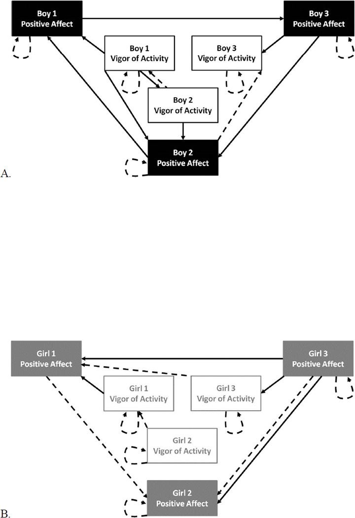
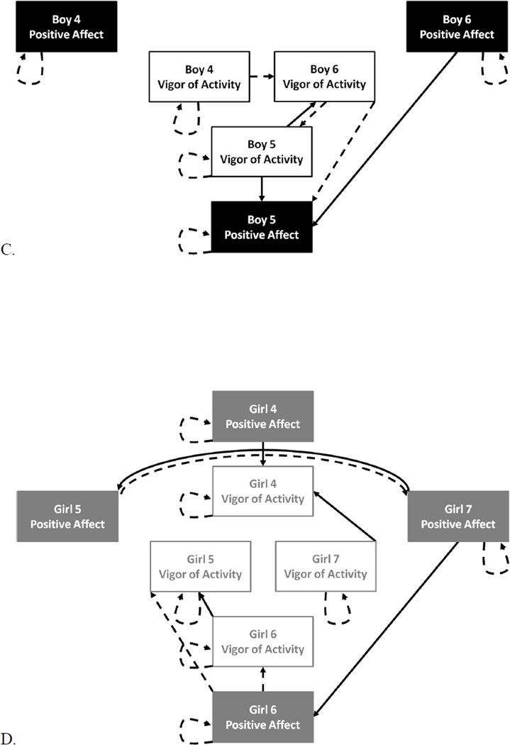
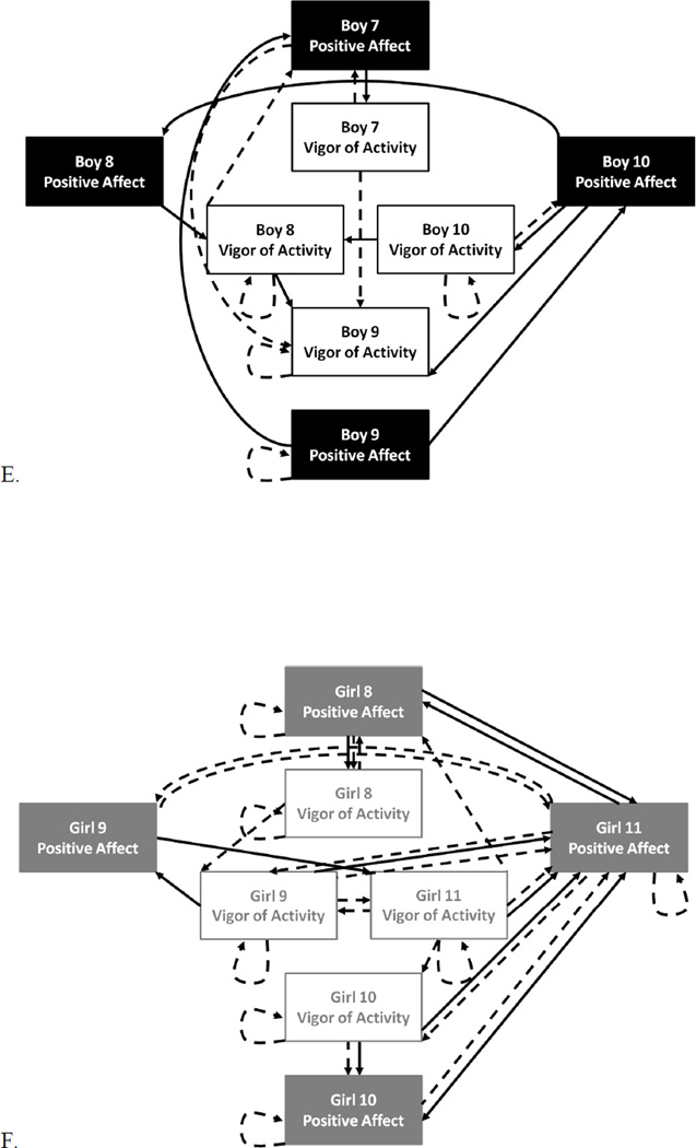
Final uSEM models for selected groups of boys (in black) and girls (in gray). Rectangles represent the time series of a behavior (positive affect or vigor of activity) for a single child, dashed arrows represent lagged relations, and solid arrows represent contemporaneous relations. The time series for each behavior of each child (coded in 10-second intervals) is explained by the time series of other modeled behaviors. For example, the positive affect of boy 1 is explained by the lagged positive affect of boy 1 (his own positive affect from 10 seconds prior), the contemporaneous vigor of activity of boy 1 (his own vigor of activity at the same time point), and the contemporaneous positive affect of boy 2 (the positive affect of boy 2 at the same time point). The presented models had excellent fit to the data:
χ2(36, N=98) = 26.87, p = .860, CFI=1.00, TLI=1.00, SRMR=.048, RMSEA=.000;
χ2(37, N=86) = 29.00, p = .820, CFI=1.00, TLI=1.00, SRMR=.055, RMSEA=.000;
χ2(40, N=91) = 37.10, p = .600, CFI=1.00, TLI=1.00, SRMR=.076, RMSEA=.000;
χ2(77, N=92) = 64.22, p = .820, CFI=1.00, TLI=1.00, SRMR=.061, RMSEA=.000;
χ2(73, N=74) = 55.70, p = .930, CFI=1.00, TLI=1.00, SRMR=.061, RMSEA=.000;
χ2(60, N=87) = 82.22, p = .0300, CFI=.98, TLI=.97, SRMR=.039, RMSEA=.066.


