Figure 1.

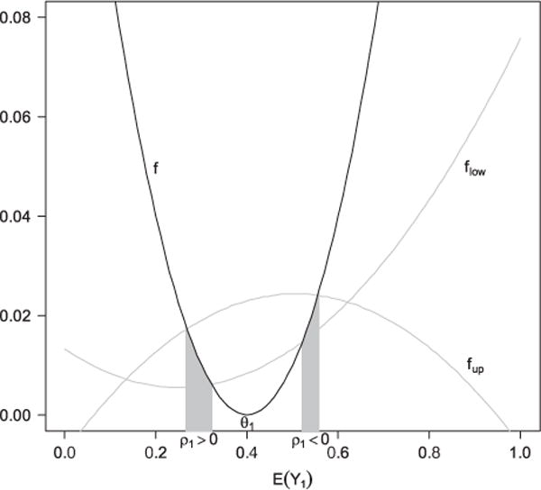
Illustration of the feasible regions of E(Y₁) defined by formula (6). f_low, f, and f_up can be viewed as three functions of E(Y₁) that correspond to the three terms in (6): $f_{\text{low}}={\text{ρ}}_1^2{\text{ν}}_1\text{ψ}\left[E\right(Y_1\left)\right(E\left(Y_1\right)-2{\text{μ}}_1)+d]$, $f={({\text{θ}}_1-E(Y_1\left)\right)}^2$, $f_{\text{up}}={\text{ρ}}_1^2{\text{ν}}_1\left[E\right(Y_1\left)\right(1-E\left(Y_1\right))-b]$.The two intervals on X-axis under the gray regions correspond to the feasible regions under ρ₁>0 and ρ₁<0, respectively. Here, θ₁= 0.4, |ρ₁| = 0.5, π = 0.5, ν₁ = 0.5, μ₁ = 0.25, ψ= 1, η₁ = 0.15, b = 0.05, and d = 0.10625.