Figure 5. Coarse-graining of the contact frequency maps and structural representation of the genome.

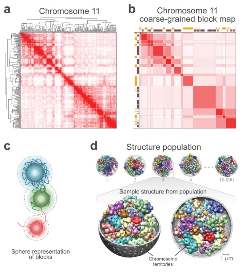
(a) The contact frequency map of chromosome 11 from the tethered HindIII library. The chromosome has been divided into 237 segments each of which covers 166 HindIII sites. Hierarchical constrained clustering was applied using the Pearson’s correlation between the segments’ contact profiles as the similarity measure (Methods). The dendrogram of constrained clustering is shown to the left and on top of the map. The intensity of the red color in each position of the map represents the observed frequency of contact between corresponding segments of the chromosome shown on the top and to the left of the map.

(b) Coarse-grained block matrix of chromosome 11. To identify the blocks, a clustering cutoff was determined following a previously described procedure³⁹. In the block map, the value of an element is the average contact frequency of all the corresponding elements in the contact frequency map. The dimension of the initial contact frequency map is reduced to 15 blocks for chromosome 11 and 428 for the entire genome in the block map. Spearman’s rank correlation coefficient between this block matrix and the contact frequency map in (a) is 0.78. Assignment of segments to the active (orange blocks) and inactive (dark brown blocks) classes are shown to the left and on top of the matrix. The intensity of the red color in each element represents the average of the observed contact frequencies between the corresponding blocks of the chromosome. See Supplementary Figure 7b-d for the coarse-grained genome-wide block matrix.

(c) Sphere representation for chromatin regions in a block. The sphere for each block is defined by two different radii. First, its hard radius (solid sphere) which is estimated from the block sequence length and nuclear occupancy of the genome; the sphere cannot be penetrated within this radius (Methods). Second, its soft radius (dotted line), which is twice that of the hard sphere radius. A contact between two spheres is defined as an overlap between the spheres’ respective soft radii. Also shown is a schematic hypothetical view of the chromatin fiber. For all the block sequence lengths and resulting sphere radii see Supplementary Table 4.

(d) Genome structure population of 10,000. A schematic of the calculated structure population is shown on top. A randomly selected sample from the population is magnified on the buttom. All forty-six chromosome territories are shown. Homologous pairs share the same color. The nuclear envelope is displayed in grey. For visualization purposes, the spheres are blurred in the magnified structure because the use of 2x428 spheres to represent the genome makes the territories appear more discrete than they actually are.