Figure 1. The prediction task.

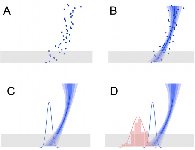
(A) On each trial, participants see a target “space invader” moving down the screen. The target appears at a series of locations in rapid succession (shown here as dots, simultaneously, for illustration) to give the impression of motion. The bottom part of the trajectory is occluded (grey box). Participants must predict where the trajectory will emerge from the occluder (trajectory endpoint). They indicate their response by moving a cursor; after they finalise their response by a button-press, feedback is given, as the target appears at its true endpoint. Trajectories are parabolic, but the start point and curvature are changed randomly on each trial. (B) The participant's estimate of the trajectory was modelled as a quadratic curve. The “best estimate” trajectory is shown here as a solid blue line; the regions indicated by the three levels of blue shading indicate the range of trajectories falling within 1, 2, and 3 standard errors from the best estimated trajectory. (C) This results in a Gaussian probabilistic estimate of the trajectory endpoint (blue bell curve). (D) The trajectory endpoints over many trials (represented by the red histogram) follow a Gaussian distribution (red bell curve), which gives some statistical information a priori about where the endpoint will be. This information can be used to reduce uncertainty in noisy trajectories. The mean and variance of this underlying distribution change periodically and must be learned using a statistical model.