Fig. 3.

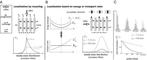
Localization of Golgi resident proteins. (A) Fast recycling of proteins imported at specific Golgi location leads to a peaked protein distribution around the import location. The steady-state distribution profile is shown for parameter values corresponding to VSVG (not a resident protein, 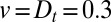, , gray curve) and for a recycling 10 times faster (black curve). (B) Local variation of the transport rates k and can be converted into energy landscapes and related to physical mechanisms, such as hydrophobic mismatch. The example shows a quadratic landscape 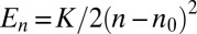and the corresponding rates. The steady-state distribution shows a peak where the net velocity vanishes. (C) Pulse-chase experiment on resident proteins in a quadratic energy landscape, showing the evolution of a protein distribution initially localized at the cis face at , and the variation of the total protein content with time. Variation of the progression velocity strongly influences the protein distribution and lifetime in the Golgi. Larger (black curve) displaces the peaks toward the trans face and promotes protein exit.