

Abstract
At an organism level, the mammalian circadian pacemaker is a two-dimensional system. For these two dimensions, phase (relative timing) and amplitude of the circadian pacemaker are commonly used. Both the phase and the amplitude (A) of the human circadian pacemaker can be observed within multiple physiological measures—including plasma cortisol, plasma melatonin, and core body temperature (CBT)—all of which are also used as markers of the circadian system. Although most previous work has concentrated on changes in phase of the circadian system, critically timed light exposure can significantly reduce the amplitude of the pacemaker. The rate at which the amplitude recovers to its equilibrium level after reduction can have physiological significance. Two mathematical models that describe the phase and amplitude dynamics of the pacemaker have been reported. These models are essentially equivalent in predictions of phase and in predictions of amplitude recovery for small changes from an equilibrium value (A = 1), but are markedly different in the prediction of recovery rates when A < 0.6. To determine which dynamic model best describes the amplitude recovery observed in experimental data; both models were fit to CBT data using a maximum likelihood procedure and compared using Akaike’s Information Criterion (AIC). For all subjects, the model with the lower recovery rate provided a better fit to data in terms of AIC, supporting evidence that the amplitude recovery of the endogenous pacemaker is slow at low amplitudes. Experiments derived from model predictions are proposed to test the influence of low amplitude recovery on the physiological and neurobehavioral functions.
Keywords: Biological Clock, Dynamic Models, Maximum Likelihood, Amplitude Recovery
INTRODUCTION
The endogenous circadian pacemaker located in the mammalian hypothalamus exerts a major influence on many physiological and neurobehavioral measures (Waterhouse and DeCoursey, 2004). Original studies of the mammalian circadian pacemaker were concerned solely with the timing (phase) of circadian processes, and to a large extent, this is still the dominant focus (Czeisler and Khalsa, 2000; Rodenbeck et al., 1998; Strogatz et al., 1986; Tilley et al., 1982). Winfree (2000) emphasized that the circadian pacemaker as a self-sustaining oscillator must have both phase as well as amplitude characteristics and demonstrated the significance of the amplitude of the pacemaker through the “strong” phase resetting process, which is termed as “Type 0” resetting. To obtain Type 0 resetting, the light stimulus must be timed to reduce the amplitude of the pacemaker to zero (singularity) or near zero, and this reduction of amplitude is both a significant as well as a necessary part of the mechanisms in producing large (~12h) phase shifts.
Type 0 resetting, originally demonstrated for Drosophila species, (Winfree, 1975) has been demonstrated in humans (Czeisler et al., 1989; Jewett et al., 1991). In humans, this concurrent amplitude reduction and phase shifting has been demonstrated using surrogate marker rhythms such as core body temperature (CBT), cortisol, and plasma melatonin levels (Jewett et al., 1991; Jewett et al., 1994; Shanahan et al., 1999). Theoretically, amplitude reduction has other physiological significances, as it can enhance phase shifting as well as result in the reduction of amplitude of physiologic functions influenced by the circadian pacemaker, including the hormones melatonin and cortisol (Shanahan et al., 1999) as well as alertness, but not all aspects of performance (Jewett and Czeisler, 1992).
Mathematical models have been developed to understand the amplitude as well as the phase of the human circadian pacemaker in functional terms (Forger et al., 1999; Jewett et al., 1999; Jewett and Kronauer, 1998; Kronauer, 1990; Kronauer et al., 1999). These models are generally used for simulation studies; however, the interaction between mathematical modelers and experimentalists can provide greater insights into the behavior of the circadian pacemaker and its output rhythms. The models can also be used for the simulation of different potential experimental protocols and to provide predictions to generate testable hypotheses for new experiments. The results of the experiments can then be used to validate and further refine the parameters of the models thereby to improve the predictive capabilities of the models.
Kronauer (1990) proposed an original mathematical model of the effects of light on the phase and amplitude of the human circadian pacemaker. This model predicted many of the general experimentally observed features of the response of the human circadian pacemaker to light (Klerman et al., 1996). The model is based on a van der Pol oscillator of cubic nonlinearity with amplitude recovery following amplitude suppression represented by a low “stiffness.” This original model has been modified as new experimental observations became available (Boivin et al., 1996; Jewett et al., 1991). Two of the recent modifications of the original model are a “higher order” model proposed by Jewett and Kronauer (1998) and a “simpler” model proposed by Forger and colleagues (1999).
Both the higher order model and simpler model are equally accurate in the prediction of phase changes in response to a light stimulus, but they differ in the prediction of amplitude changes of the pacemaker following amplitude suppression. The higher order model employs a van der Pol type function of higher order nonlinearity with the same stiffness as the original model; whereas, the simpler model includes cubic nonlinearity of the original model with enhanced stiffness. As a result, the amplitude recovery following a critical stimulus is slower at low amplitudes in the higher order model than in the simpler model. However, neither of these dynamic models has been carefully validated using experimental data with low circadian amplitude. Therefore, we compared these two different dynamic models using CBT data to determine which model provides a better fit to experimental data in terms of amplitude recovery.
CBT data are a reliable marker of the circadian pacemaker that can be monitored continuously in real time with a high sampling rate. However, a disadvantage of CBT data is that they also contain statistical fluctuations due to the body’s thermoregulatory response and other physiological factors. Under appropriate experimental protocols, such as the Constant Routine (CR) protocol (described below), these other physiological factors can be minimized, leaving a variable containing only circadian and thermoregulatory components (Duffy, 1993). To address the question of which dynamic model best describes the amplitude recovery of the circadian pacemaker at low amplitudes, we used a method proposed by Brown and coworkers (2000) to fit the two models to the experimental data. With this method, each dynamic model is integrated within a statistical framework and is fit to CBT data using a maximum likelihood approach. The goodness-of-fit measure is used to compare the models.
MATERIALS AND METHODS
Mathematical Models of the Human Circadian Pacemaker
The mathematical models of the human circadian pacemaker (Forger et al., 1999; Jewett et al., 1999; Kronauer et al., 1999; Kronauer et al., 2000) to be compared both have two distinct dynamic units (Figure 1): Process L, a stimulus preprocessor that converts the light input I(t) into the drive B̂(t), and Process P, a circadian pacemaker unit that has a two-dimensional self-sustaining Limit Cycle Oscillator (LCO), and a Sensitivity Modulator (SM). The SM adjusts the strength of B̂(t), depending on circadian pacemaker variables to produce the drive B(t), that then acts to shift phase and amplitude. The mathematical equations for the SM and Process L are the same both for higher order and simpler models.
FIGURE 1.

Schematic diagram of the model of the effect of light on the human circadian pacemaker: Light (I) enters the dynamic stimulus processor (Process L), where it activates a group of elements to produce a drive B̂ onto the human circadian pacemaker (Process P). This drive then enters a circadian stimulus modulator (SM) that reduces or enhances the strength of the light drive B̂, depending on the phase of the circadian pacemaker, to produce a modulated drive B. This modulated light drive then acts on the pacemaker, modeled by a limit-cycle oscillator (LCO), altering the phase and amplitude of the circadian pacemaker via the two state variables x and xc.
Process L represents the photic input pathway of the circadian system. This preprocessor intervenes between light and the pacemaker to provide an input to the pacemaker with strong initial drive followed by a sustained drive for longer-duration light stimuli.
Process L comprises many activator elements that can be either in a “used” state (with probability n) or in a “ready” state (with probability 1 − n). Light activates the ready elements and delivers a drive to the Process P, after which the elements enter the used state, from which they can be recycled back to the ready state. The dynamic equation that represents Process L is:
| (1) |
where α is the activation rate and β is a recycling constant. This equation is incorporated to predict the response of circadian pacemaker due to intermittent light pulses according to experimental observation (Rimmer et al., 2000).
The activation rate α depends on light intensity I(t) according to a power-law:
| (2) |
with α0 = 0.05, p = 0.5 as the characteristic exponent (Boivin et al., 1996) and Io = 9500 lux.
The drive B̂(t) is represented as:
| (3) |
where G is a scaling constant.
The SM transforms B̂(t) to B(t), which acts as an input to the limit cycle oscillator and is represented as:
| (4) |
Equation (4), along with equations (1), (2), and (3), may be interpreted as a modulation of photic sensitivity of the oscillator according to circadian phase.
Process P is the oscillator unit generating the circadian rhythm with outputs to measurable physiologic functions.
The LCO in Process P for the higher order model is expressed mathematically as:
| (5) |
| (6) |
τx is the period of the circadian oscillator, which varies between subjects and averages 24.2 h (Brown et al., 2004; Czeisler et al., 1999), stiffness μ is set at 0.13; k = 0.55 and q = 1/3.
The LCO for the simpler model is expressed as
| (7) |
| (8) |
Note that equation 8 shows the cubic nonlinearity of the original model (Kronauer, 1990) but with enhanced stiffness μ = 0.23. The simpler model does not contain a secondary divergence term qBxc as seen in equation 6 for the higher order model. The divergence term was included in the higher order model to accommodate the extreme precision with which stimuli must be timed to generate amplitude reduction.
Theoretical Calculation of Growth
We determine the amplitude of the pacemaker for both models using:
| (9) |
Using the method of averaging (Andronov et al., 1966), the change of amplitude over one cycle ΔA can be calculated. For the simpler model, we find the classic van der Pol result:
| (10) |
where Ā is the average amplitude for the particular cycle.
For the higher order model we obtained:
| (11) |
Since we are interested in the behavior of the models at low-amplitudes, it is useful to introduce a normalized growth, GI, defined as:
| (12) |
along with suffixes to denote the separate models:
| (13) |
These models differ significantly in their prediction of growth at low amplitudes (Figure 2), especially with the assigned values μS = 0.23 (Forger et al., 1999) and μH = 0.13 (Jewett and Kronauer, 1998).
FIGURE 2.
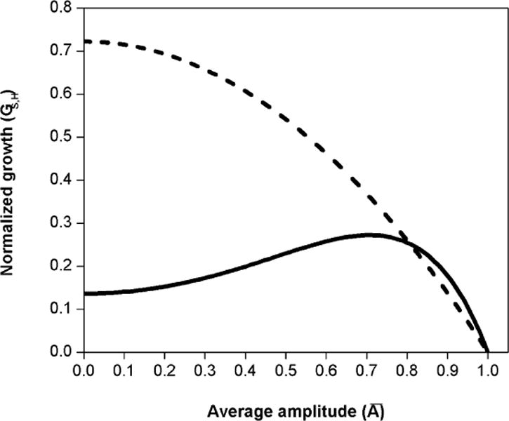
Theoretical normalized growth for simpler model (GS, dashed line) and higher order model (GH, solid line), for the average amplitudes between (singularity) and (limit cycle) at 0 lux. The recovery of the amplitude in the higher order model is slower near the singularity than in the simpler model. The models have similar predictions of growth near the limit cycle.
Integration of Dynamic and Statistical Models
To perform the comparisons between the two dynamic models, we represented these models on a statistical modeling framework using the procedure in Brown and colleagues (2000). CBT data, yn, were measured during CR at evenly spaced (1 min) intervals of n = 1,2,…, N. The data yn thus collected were represented as the sum of circadian and thermoregulatory processes:
| (14) |
where xn is the circadian component, and υn is the fluctuation in CBT due to the thermoregulatory response to random excitation.
The circadian system xn is obtained by numerical integration of either higher order model, as in equations (5) and (6) above, or simpler model, as in equations (7) and (8) above. Since there is no known interaction between circadian and thermoregulatory systems, the υn are here represented as an independent first-order autoregressive [AR(1)] process defined as
| (15) |
where ρ is the coefficient of the AR(1) process and the residual εn are independent, Gaussian random variables with zero mean and variance . The sampling time Δt is set at 0.1 h (6 min) for increasing the estimation precision of ρ; for details refer Brown and Czeisler (1992).
We fit the model in equation 14 by a maximum likelihood method with the Gaussian assumption for υn and defining the log likelihood (Brown et al., 2000) for either model as
| (16) |
Here |Γ(ρ)| is the determinant of the covariance matrix of the AR(1) process and
| (17) |
where θ is the vector of initial conditions of models, xo and xco. The parameters θ and ρ are estimated by a nonlinear optimization of LN (Brown and Schmid, 1994; Jones, 1980). Since each data set is fitted to the model by maximizing the likelihood function, we compared results between the models by the Akaike’s Information Criterion (AIC) that explicitly embodies the likelihood:
| (18) |
The model with the lower AIC is considered the better model. AIC is accepted as one of the most reliable methods for comparing different classes of models in model fitting (Priestley, 2001).
Analysis Procedure
We used CBT data collected from 14 healthy subjects; the experiments were fully described in Jewett and colleagues (1994). The constant routine (CR) procedure is used to minimize the evoked effects of sleep, light, postural changes, and activity on CBT (Duffy, 1993). During a CR, a subject remains awake in dim light in a semi-recumbent posture with frequent small meals. This minimizes evoked effects on CBT so that our assumption of CBT reflecting only circadian and thermoregulatory components is valid. A pre-stimulus CR (CR1) for each subject was used to provide an assessment of the equilibrium (limit cycle) amplitude of the endogenous circadian pacemaker and the time of CBT minimum (CBTmin), the marker of circadian phase. The subjects were then exposed to a stimulus of bright light (7000 to 12,000 lux) near the CBTmin to produce amplitude suppression. A second CR (CR2) was conducted after this stimulus, during which circadian phase and amplitude were again assessed. The CRs were conducted using a room light level of 150 lux, except for one subject (1027 v), who was exposed to 0 lux (total darkness) during CR2.
Of the 14 original subjects, data from four subjects were not included in the final analysis. In one of these subjects, ~16% of CBT data in CR2 were missing, while in the three other subjects, the normalized amplitudes in CR2 were close to 1.0 (the limit cycle), indicating amplitude suppression had not been induced. Therefore, data from 10 subjects were used in this analysis.
It was assumed that the CBT amplitude oscillation from the mean temperature value during CR1 was at the limit cycle (equilibrium); however, this amplitude was different for the different subjects (Jewett et al., 1991). Therefore, the dynamic equations for both models were scaled with the estimated amplitude at CR1 using the procedure described by Brown and colleagues (2000). This scaling procedure would help to determine the amplitude at CR2 considering amplitude at CR1 as the limit cycle. The scaled equations were then fit to the data of CR2. The final fitting procedure yields three parameters for each model. The first two parameters are the initial conditions (xo, xco) from which the dynamic equations are numerically integrated; the third parameter is the coefficient (ρ) of the autoregressive process.
We analyzed the residuals using power spectral analysis (Priestley, 2001) to determine whether our procedure could capture most of the important structure in the data. We compared the models quantitatively using AIC. For both representations of the dynamic models, the number of estimated parameters is three (xo, xco, ρ). Hence, any difference in AIC between the models is a direct measure of likelihood. We evaluated the relation between change in growth (ΔG) predicted by these models and change in estimated AIC (ΔAIC) of the model by finding an appropriate relation between ΔG and ΔAIC using a best-fit procedure. We also compared the model predictions by designing two experimental protocols. One of the experimental protocols is designed to simulate the amplitude recovery and the other protocol is designed to study the effect of light on phase shifting at low amplitudes. Results from these protocols can be used to compare model predictions and understand the effects of changing circadian amplitude on different physiological as well as neurological measures.
RESULTS
Model Fits to Data
Both models fit the data well in terms of graphical goodness of fit (Figure 3). The AR(1) process captured the statistical characteristics of the body’s thermoregulatory response. As an example, the estimated circadian signal of the models along with the original CBT data of subject 1027 v is shown in Figure 3(a). Data from this subject were chosen because they demonstrate the largest difference in AIC between the models. Note that the higher order model predicts a slower recovery of amplitude than the simpler model, as would be expected with a lower stiffness and higher order nonlinearity. Figure 3(b and c) shows the estimated thermoregulatory component captured by the AR(1) process along with the residuals. The magnitude of the residuals is small indicating that AR process captures statistical fluctuations in the data for this subject. The estimated variance of the residuals is on the order of ~10−4 (approximately 1/100 of the CBT amplitude of 10−2) for all subjects for both models (Table 1). In addition there were no statistically significant spectral components in power spectral density of the residual series. We therefore concluded that our integrated procedure captured both the statistical and dynamic structure in the CBT data.
FIGURE 3.
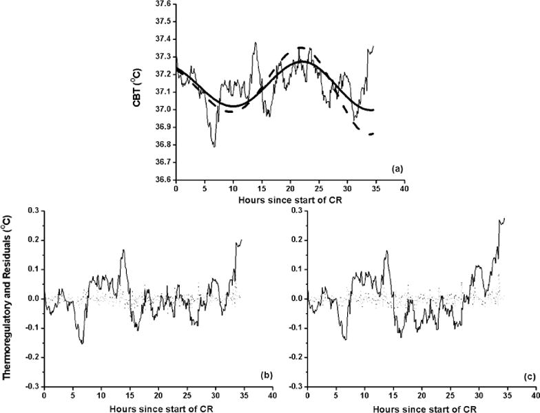
(a) Estimated circadian signal of the higher order (solid line) and simpler model (dashed line) to CBT of subject 1027v during a constant routine (CR2) in 0 lux following amplitude suppression due to bright light stimulus. The amplitude at CR1 is 37.14 ± 0.29. The higher order model predicts slower amplitude growth than the simpler model. Estimations of the thermoregulatory component (solid line, panels b and c) and residuals (dots, panels b and c) were made using the integrated procedure with higher order model (b) and simpler model (c) as the limit cycle oscillator of Process P.
TABLE 1.
The Variance of the Residuals , Average Normalized Amplitudes ( and ), the Corresponding Normalized Growths (GS and GH), AIC for Each Mathematical Model (AICS and AICH) for Each Subject and Difference in AIC (ΔAIC = AICH − AICS)
| Simpler model
|
Higher order model
|
||||||||||||
|---|---|---|---|---|---|---|---|---|---|---|---|---|---|
| Subject |
|
|
GS | AICS |
|
|
GH | AICH | ΔAIC | ||||
| 642v | 3.8406 | 0.24 | 0.54 | −276.78 | 3.8343 | 0.23 | 0.16 | −277.24 | −0.46 | ||||
| 703v7t2 v | 2.8701 | 0.23 | 0.53 | −384.49 | 2.8598 | 0.23 | 0.17 | −385.71 | −1.22 | ||||
| 724v | 4.6439 | 0.54 | 0.40 | −200.02 | 4.6381 | 0.47 | 0.23 | −200.69 | −0.67 | ||||
| 831v | 3.3844 | 0.17 | 0.55 | −313.21 | 3.382 | 0.18 | 0.16 | −313.54 | −0.33 | ||||
| 914v | 6.8226 | 0.39 | 0.47 | −83.35 | 6.7896 | 0.35 | 0.19 | −84.97 | −1.62 | ||||
| 916v | 2.7885 | 0.55 | 0.39 | −395.79 | 2.7828 | 0.47 | 0.23 | −396.66 | −0.87 | ||||
| 917v | 2.0193 | 0.32 | 0.50 | −500.69 | 2.0034 | 0.29 | 0.18 | −503.31 | −2.62 | ||||
| 919v | 7.7734 | 0.60 | 0.34 | −37.31 | 7.7676 | 0.57 | 0.25 | −37.57 | −0.26 | ||||
| 926v | 2.4879 | 0.40 | 0.46 | −438.36 | 2.4656 | 0.32 | 0.19 | −441.51 | −3.15 | ||||
| 1027 v | 3.3655 | 0.37 | 0.60 | −330.83 | 3.3237 | 0.25 | 0.16 | −335.46 | −4.63 | ||||
For all 10 subjects, the AIC of the higher order model was lower than the AIC of the simpler model, suggesting that the higher order model, which has a slower growth, provides a better fit to the data. Due to the slower growth, the average amplitude of higher order model was ~13% less than the average amplitude of simpler model during CR2 (Table 1). The normalized growth of the simpler model (GS) is also considerably larger than the growth of the higher order model (GH) at low amplitudes.
Relation Between ΔG and ΔAIC
Since the two models differ in their growth at low amplitudes, we explored the relationship between the estimated difference in growth, ΔG = GS − GH, to the difference in AIC, ΔAIC = AICH − AICS. The relationship between the change in the goodness of fit measure, ΔAIC, and the change in dynamic property of the model, ΔG, can be used to determine whether our methodology is correct and if a relation exists, can eventually help to further refine the mathematical models. Therefore, first we computed ΔG and ΔAIC with respect to the circadian amplitude calculated from each of the models. Due to the lack of the divergence term (qBxc) in the simpler model, equation (10) has to be scaled by a factor of 0.8 to accommodate the effect of 150 lux on growth of the pacemaker amplitude (Forger et al., 1999). Since the estimated average amplitudes of the models are different, we define reference amplitude AR as the mean of and for each subject. The estimated ΔG for each subject along with theoretical ΔG obtained from the method of averaging (Andronov et al., 1966) are shown in Figure 4a. There is little difference graphically between the estimated and theoretical ΔGs, which supports the validity of our methodology. The difference in growth between the models is greatest at low amplitudes, which is consistent with the predictions derived from the theoretical analysis of the models (e.g., Figure 2). As the amplitude increases, ΔG between the simpler and higher order model decreases, consistent with the finding that the models predict similar growth at higher amplitudes. The ΔG becomes zero at amplitude AR ~ 0.74.
FIGURE 4.
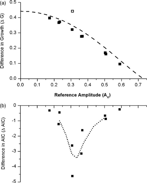
(a) The estimated difference in growth ΔG, (GS − GH), in individual subjects (closed boxes) compared with theoretical ΔG (dashed line) at a room light of 150 lux. The open square represents subject 1027 v, who was at 0 lux during CR2. (b) The difference in AIC, ΔAIC = AICH − AICS, of the higher order model and simpler model with respect to a reference amplitude AR. A 3-point smoothing (dotted line) suggests ΔAIC → 0 as AR → 0 and AR → 0.7.
We also plotted the difference in AIC, ΔAIC = AICH − AICS, with respect to the reference amplitude (Figure 4b). Unlike the relationship between ΔG and AR, ΔAIC has a biphasic relationship with a minimum at AR ~ 0.3. Both ΔG and ΔAIC tend to zero at AR ~ 0.74. Under the current experimental conditions, the lowest recorded pacemaker amplitude is A = 0.17, and hence we are unable to predict the behavior at lower amplitudes. However, a three-point smoothing procedure (dotted line in Figure 4b) suggests that ΔAIC → 0 as AR → 0, suggesting that both the higher order and simpler model have similar predictions at these very low amplitudes.
Proposed Experiments
After comparing the models to experimental data, we used these two models to design two experimental protocols to generate testable hypothesis to further test the models as well as to better understand the impact of circadian amplitude on neurobehavioral performance and circadian phase shifting. These protocols are a modification of the existing experimental protocols described in Czeisler and colleagues (1989) and Jewett and coworkers (1991). The first experiment is designed specifically to understand the significance of low amplitude on neurobehavioral measures influenced by the circadian pacemaker, whereas the second experiment is designed to study the effect of phase-shifting at low amplitudes on these measures.
During both protocols, multiple marker variables should be used (e.g., CBT, cortisol and melatonin) with frequent sampling to assess circadian phase and amplitude. Change in amplitude in more than one marker variable demonstrates the change in amplitude of the endogenous circadian pacemaker rather than change in marker amplitude downstream from the pacemaker. For the practical applications to work and worker safety, multiple neurobehavioral performance and subjective alertness measurements should be made frequently when the subject is awake to assess the effects of amplitude reduction of the circadian pacemaker. These studies also need to be done on younger and older persons, since the amplitude of the pacemaker is lower in many older persons (Czeisler et al., 1992), and this effect of decreased pre-stimulus amplitude should be assessed.
In the first experimental protocol, there are three 24 h baseline cycles (Three 8h, 0 lux sleep episodes and two 16 h, 150 lux wake episodes) followed by a CR (CR1) in 10 lux to assess circadian phase. The length of the CR will depend on each individual subject’s circadian phase. The CR must be of such a length so that the center of the light pulse following CR1 occurs directly at the minimum of CBT (CBTmin), as determined during CR1. One light pulse of 10,000 lux of 6.5 h duration centered in the middle of waking day is applied each day on two consecutive days with the center of the pulse falling at CBTmin. These two days are followed by a post-stimulus CR (CR2) to assess the final circadian phase and amplitude. CR2 is followed by 3 recovery days in 10 lux. The waking background lux level has been reduced in these proposed experiments from that of previous studies (Boivin et al., 1996; Rimmer et al., 2000) to eliminate the possibility of confounding the results by phase-shifts produced by the background light (even ~150 lux). The second experimental protocol is similar to the first one; with a third 6.5 h, 10,000 lux stimulus is applied following CR2 with the pulse centered 3 h after the CBTmin recorded at CR1. This is then followed by another CR (CR3) to assess circadian phase and amplitude.
The schematic of the experimental protocol and predictions of the models are shown in Figure 5. In the first experiment (left panel) the amplitudes of the higher order model and simpler model calculated using equation (9) suppress to a value of 0.20 and 0.15, respectively, shortly after the two-pulse stimulus. During CR2 the model predicts that the amplitude reaches a peak value of 0.22 and 0.30, respectively. However, instead of recovering, the amplitude of the higher order model suppresses during the recovery days, whereas the amplitude of the simpler model recovers to a value of 0.91. The results of this proposed experimental protocol should both test these predictions as we compare the models and help to understand the significance of low amplitude recovery on neurobehavioral performance and on circadian phase shifting.
FIGURE 5.
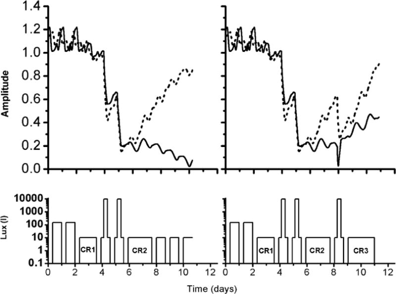
Comparisons of the amplitude predictions of higher order model (solid line) and simpler model (dashed line) in two experimental protocols designed to suppress amplitude. Left panel: Experimental protocol 1 (bottom) in which 2 consecutive cycles of light pulses are administered such that the center of the light pulses coincides with the CBTmin as recorded during a pre-stimulus CR (CR1). Right panel: Experimental protocol 2, (bottom), which is similar to the protocol 1, except with the addition of a third light pulse scheduled following CR2 such that the center of the pulse falls 3h after CBTmin as recorded during CR1.
In the second experiment (right panel), the higher order model predicts that the third light pulse produces a phase advance of ~7.7h, whereas the simpler model predicts a phase advance of ~0.8h. In addition, both models predict recovery of the amplitude of the circadian pacemaker instead of suppressing as observed in the first experiment. The final predicted amplitudes are 0.7 for the higher order model and 0.8 for the simpler model. This experimental protocol would help us to determine whether the low amplitude would enhance phase shifting.
DISCUSSION
Since both amplitude and phase are required to define the two-dimensions of the circadian pacemaker, it is of considerable interest to quantify the rate of amplitude recovery when circadian amplitude is suppressed. Mathematical models reflecting different underlying physiologies can be used to predict the amplitude recovery dynamics of the endogenous circadian pacemaker. We compared the performance of two recently developed mathematical models of the human circadian pacemaker that have different predictions of amplitude recovery to study which model best describes the experimental data in terms of amplitude recovery. We also used these models to design experiments to further define the physiology as well as to further differentiate the model predictions as a part of the ongoing experiment-mathematical model-experiment paradigm.
Based on the analysis of experimental data, we found that the model with slow growth (higher order model) provided a better fit to the data in terms of the AIC. Based on this observation, we predict that, due to slow amplitude recovery of the circadian pacemaker, the circadian component of alertness and performance will also be recovered slowly to an equilibrium value after an amplitude-reducing stimulus. This prediction needs to be tested, especially since both the absolute level of alertness as well as performance and the rate of change may be important. Furthermore, the light stimulus applied during slow recovery can enhance phase shifting. We proposed experiments to test these predictions.
We found from the relation between ΔAIC and ΔG that the larger the difference in growth between the models, the better the prediction by the slow-growth model. However this feature is seen only in the amplitude region 0.3 < AR < 0.75. At amplitudes AR < 0.3 ΔG are larger and one might anticipate large ΔAIC. However we found that ΔAIC is smaller at these amplitudes in comparison with other ones. This implies that related, but as yet undeveloped, mathematical models with slower growth rates than the higher order model potentially could provide better fit to the experimental data at these very low relative amplitudes. To characterize the growth accurately from data, we need to estimate directly the parameters in the equations corresponding to growth, i.e., the stiffness and the coefficients of the higher-order polynomial using this same modeling framework. Also needed are more experiments at low light levels as well as at lower amplitudes of the circadian pacemaker to accurately characterize the growth of the endogenous circadian pacemaker as well as the behavior of the system at low amplitudes.
Dynamic models are generally designed to predict the qualitative characteristics of the circadian pacemaker, and the parameters of the model frequently are selected to simulate these characteristics without using formal statistical methods. The significance of our analysis is that we implemented a procedure to integrate the dynamic models on a statistical modeling framework such that the parameters of the model can be estimated directly from the experimental data. In this analysis, two types of dynamic models with different amplitude characteristics are compared on a statistical framework by estimating only the initial conditions of the dynamic models. However, this procedure can also be used to determine the other parameters of the dynamic model directly from the data, thereby providing quantitative inferences about the behavior of the pacemaker.
A key feature of our work is that we demonstrate the significance of validating dynamic models using experimental data as well as designing new experimental protocols using models to further understand the physiology. Using mathematical models to design experiments and the results of experiments to refine mathematical models should be efficient as well as productive in understanding the effect of amplitude of the circadian pacemaker on different physiological and neurobehavioral measures.
Acknowledgments
We thank Drs Charles A. Czeisler, Jeanne F. Duffy, and Theresa L. Shanahan for sharing their insights on experimental protocols and to Luana Delvecchio for administrative assistance. This work was supported in part by National Aeronautics and Space Administration Cooperative Agreement NCC 9–58 with the National Space Biomedical Research Institute, grants F30602-01-2-0554 of Defense Advanced Research Projects Agency, P01-AG00975 of National Institute of Mental Health, R01-GM53559 of National Institute General Medical Sciences and NCRR-GCRC-MO1-RR02635 of National Institute of Health. EBK is supported by NIH grant K02-HD045459.
References
- Andronov AA, Vitt AA, Khaikin SE. Theory of Oscillators. New York: Dover Publications; 1966. [Google Scholar]
- Boivin DB, Duffy JF, Kronauer RE, Czeisler CA. Dose-response relationships for resetting of human circadian clock by light. Nature. 1996;379:585–613. doi: 10.1038/379540a0. [DOI] [PubMed] [Google Scholar]
- Brown EN, Czeisler CA. The statistical analysis of circadian phase and amplitude in constant routine core temperature data. J Biol Rhythms. 1992;7:177–189. doi: 10.1177/074873049200700301. [DOI] [PubMed] [Google Scholar]
- Brown EN, Schmid CH. Application of the Kalman filter to computational problems in statistics. In: Brand L, Johnson ML, editors. Methods in Enzymology, Numerical Computer Methods, Part B. Orlando: Academic Press; 1994. pp. 171–181. [DOI] [PubMed] [Google Scholar]
- Brown EN, Choe Y, Luithardt H, Czeisler CA. A statistical model of the human core-temperature circadian rhythm. Am J Physiol Endocrinol Metab. 2000;279:E669–E683. doi: 10.1152/ajpendo.2000.279.3.E669. [DOI] [PubMed] [Google Scholar]
- Brown EN, Solo V, Zhang Z. Measuring the period of the human biological clock. In: Brand L, Johnson ML, editors. Methods in Enzymology, Numerical Computer Methods. Vol. 383. Orlando: Academic Press; 2004. pp. 383–405. [DOI] [PubMed] [Google Scholar]
- Czeisler CA, Khalsa SBS. The human circadian timing system and sleep-wake regulation. In: Kryger MH, Roth T, Dement WC, editors. Principles and Practice of Sleep Medicine. Philadelphia: W.B. Saunders Company; 2000. pp. 353–374. [Google Scholar]
- Czeisler CA, Kronauer RE, Allan JS, Duffy JF, Jewett ME, Brown EN, Ronda JM. Bright light induction of strong (type 0) resetting of the human circadian pacemaker. Science. 1989;244:1328–1333. doi: 10.1126/science.2734611. [DOI] [PubMed] [Google Scholar]
- Czeisler CA, Dumont M, Duffy JF, Steinberg JD, Richardson GS, Brown EN, Sánchez R, Ríos CD, Ronda JM. Association of sleep-wake habits in older people with changes in output of circadian pacemaker. Lancet. 1992;340:933–936. doi: 10.1016/0140-6736(92)92817-y. [DOI] [PubMed] [Google Scholar]
- Czeisler CA, Duffy JF, Shanahan TL, Brown EN, Mitchell JF, Rimmer DW, Ronda JM, Silva EJ, Allan JS, Emens JS, Dijk DJ, Kronauer RE. Stability, precision, and near-24-hour period of the human circadian pacemaker. Science. 1999;284:2177–2181. doi: 10.1126/science.284.5423.2177. [DOI] [PubMed] [Google Scholar]
- Duffy JF. Constant routine. In: Carskadon MA, editor. Encyclopedia of Sleep and Dreaming. New York: Macmillan Publishing Company; 1993. pp. 134–136. [Google Scholar]
- Forger DB, Jewett ME, Kronauer RE. A simpler model of the human circadian clock. J Biol Rhythms. 1999;14:532–537. doi: 10.1177/074873099129000867. [DOI] [PubMed] [Google Scholar]
- Jewett ME, Czeisler CA. The role of endogenous circadian amplitude in the modulation of alertness and performance: an investigation of the singular region. Sleep Res. 1992;21:378. [Google Scholar]
- Jewett ME, Kronauer RE. Refinement of a limit cycle oscillator model of the effects of light on the human circadian pacemaker. J Theor Biol. 1998;192:455–465. doi: 10.1006/jtbi.1998.0667. [DOI] [PubMed] [Google Scholar]
- Jewett ME, Kronauer RE, Czeisler CA. Light-induced suppression of endogenous circadian amplitude in humans. Nature. 1991;350:59–62. doi: 10.1038/350059a0. [DOI] [PubMed] [Google Scholar]
- Jewett ME, Kronauer RE, Czeisler CA. Phase/amplitude resetting of the human circadian pacemaker via bright light: a further analysis. J Biol Rhythms. 1994;9:295–314. doi: 10.1177/074873049400900310. [DOI] [PubMed] [Google Scholar]
- Jewett ME, Forger DB, Kronauer RE. Revised limit cycle oscillator model of human circadian pacemaker. J Biol Rhythms. 1999;14:493–499. doi: 10.1177/074873049901400608. [DOI] [PubMed] [Google Scholar]
- Jones RH. Maximum likelihood fitting of ARMA models to time series with missing observations. Technometrics. 1980;22:389–395. [Google Scholar]
- Klerman EB, Dijk DJ, Kronauer RE, Czeisler CA. Simulations of light effects on the human circadian pacemaker: implications for assessment of intrinsic period. Am J Physiol. 1996;270:R271–R282. doi: 10.1152/ajpregu.1996.270.1.R271. [DOI] [PubMed] [Google Scholar]
- Kronauer RE. A quantitative model for the effects of light on the amplitude and phase of the deep circadian pacemaker, based on human data. In: Horne J, editor. Sleep ’90, Proceedings of the Tenth European Congress on Sleep Research. Dusseldorf: Pontenagel Press; 1990. pp. 306–309. [Google Scholar]
- Kronauer RE, Forger DB, Jewett ME. Quantifying human circadian pacemaker response to brief, extended, and repeated light stimuli over the photopic range. J Biol Rhythms. 1999;14:500–515. doi: 10.1177/074873099129001073. [DOI] [PubMed] [Google Scholar]
- Kronauer RE, Forger DB, Jewett ME. Errata Quantifying human circadian pacemaker response to brief, extended, and repeated light stimuli over the photopic range. J Biol Rhythms. 2000;15:184–186. doi: 10.1177/074873099129001073. [DOI] [PubMed] [Google Scholar]
- Priestley MB. Spectral Analysis and Time Series. London: Academic Press; 2001. pp. 367–370. [Google Scholar]
- Rimmer DW, Boivin DB, Shanahan TL, Kronauer RE, Duffy JF, Czeisler CA. Dynamic resetting of the human circadian pacemaker by intermittent bright light. Am J Physiol Regul Integr Comp Physiol. 2000;279:R1574–R1579. doi: 10.1152/ajpregu.2000.279.5.R1574. [DOI] [PubMed] [Google Scholar]
- Rodenbeck A, Huether G, Ruther E, Hajak G. Altered circadian melatonin secretion patterns in relation to sleep in patients with chronic sleep-wake rhythm disorders. J Pineal Res. 1998;25:201–210. doi: 10.1111/j.1600-079x.1998.tb00389.x. [DOI] [PubMed] [Google Scholar]
- Shanahan TL, Kronauer RE, Duffy JF, Williams GH, Czeisler CA. Melatonin rhythm observed throughout a three-cycle bright-light stimulus designed to reset the human circadian pacemaker. J Biol Rhythms. 1999;14:237–253. doi: 10.1177/074873099129000560. [DOI] [PubMed] [Google Scholar]
- Strogatz SH, Kronauer RE, Czeisler CA. Circadian regulation dominates homeostatic control of sleep length and prior wake length in humans. Sleep. 1986;9:353–364. doi: 10.1093/sleep/9.2.353. [DOI] [PubMed] [Google Scholar]
- Tilley AJ, Wilkinson RT, Warren PSG, Watson B, Drud M. The sleep and performance of shift workers. Hum Factors. 1982;24:629–641. doi: 10.1177/001872088202400601. [DOI] [PubMed] [Google Scholar]
- Waterhouse JM, DeCoursey PJ. Human circadian organization. In: Dunlap JC, Loros JJ, DeCoursey PJ, editors. Chronobiology: Biological Timekeeping. Sunderland: Sinauer Associates; 2004. pp. 291–324. [Google Scholar]
- Winfree AT. Resetting biological clocks. Phys Today. 1975;28:34–39. [Google Scholar]
- Winfree AT. The Geometry of Biological Time. New York: Springer; 2000. pp. 592–600. [Google Scholar]