Bayesian Scalar-on-Image Regression with Application to Association Between Intracranial DTI and Cognitive Outcomes

Abstract

Diffusion tensor imaging (DTI) measures water diffusion within white matter, allowing for in vivo quantification of brain pathways. These pathways often subserve specific functions, and impairment of those functions is often associated with imaging abnormalities. As a method for predicting clinical disability from DTI images, we propose a hierarchical Bayesian “scalar-on-image” regression procedure. Our procedure introduces a latent binary map that estimates the locations of predictive voxels and penalizes the magnitude of effect sizes in these voxels, thereby resolving the ill-posed nature of the problem. By inducing a spatial prior structure, the procedure yields a sparse association map that also maintains spatial continuity of predictive regions. The method is demonstrated on a simulation study and on a study of association between fractional anisotropy and cognitive disability in a cross-sectional sample of 135 multiple sclerosis patients.

Introduction

Diffusion tensor imaging is a technique to quantify white matter pathways in the brain and spinal cord in vivo. In clinical applications, it opens the possibility to investigate the relationship between abnormal brain anatomy and neurological diseases [Ciccarelli et al., 2008]. For example, several studies show that DTI can produce MRI indices in specific white matter tracts that may be associated with clinical disability in multiple sclerosis (MS), a disease that causes severe motor and cognitive deficits [Kern et al., 2010; Lin et al., 2008, 2005; Lowe et al., 2006; Ozturk et al., 2010].

These studies provide important insights into the organization of the brain and the effect of brain disorders. Results may be used as a tool for the diagnosis and management of patient care or as surrogate markers in future clinical trials, particularly if they are shown to be pharmacologically sensitive. However, some clinical researchers question the implications of these study results, because the correlations between current MRI measures and clinical disability, although significant, have generally been low [Barkhof, 2002; Goodin, 2006]. Such small correlations may be due to the intrinsic variability in the clinical expression of MS plaques in various anatomical locations.

Voxel-wise or mass-univariate regression, often referred to as the “general linear model”, is a standard technique for exploring the relationship between images and scalar measures such as clinical disability scores. In this approach, one regresses brain structure measurements on a disability score separately at each voxel [Ashburner and Friston, 2000; Smith et al., 2006] to produce a statistical parametric map [Friston et al., 1994]. Such maps open the door to localizing the voxels that are significantly related to disability. Thresholded version of the resulting maps may also be used to predict disability scores [Efron, 2009; Purcell et al., 2009]. However, mass-univariate estimation treats each voxel as independent, as opposed to sharing information across neighboring voxels.

Multivariate or “decoding” models [e.g. Haxby et al., 2001; Haynes and Rees, 2006; Norman et al., 2006] seek to overcome these limitations. One such model that incorporates complex spatial structure is scalar-on-function regression [Goldsmith et al., 2011], in which the outcome is regressed on an entire one-dimensional white matter tract profile at once. This approach uses a weighted version of the tract profile, where the weights are estimated from the data. A useful by-product of the fitting algorithm is a tract-specific disability index, which is easy to understand and analyze. The method was developed for hundreds or thousands of locations along a neuronal tract, but it is not well suited for: 1) scaling up to tens or hundreds of thousands of locations; 2) modeling response surfaces that can be sparse and with abrupt edges; and 3) adapting to 3-D brain geometry, which contains complex manifold structures that are imperfectly observed.

In this paper we introduce a scalar-on-image regression method for studying the association between clinical measures and 3D brain maps. The method is computationally efficient, can be carried out over a large region of the brain, and can be adapted to highly irregular brain regions using a flexible spatial neighborhood definition. The term “scalar-on-image regression”, analogous to the nomenclature of Reiss et al. [2011], refers to the fact that whereas the responses are scalars as in conventional regression, the predictors are entire images. This method provides a coefficient image that describes the association between each voxel and the outcome, adjusting for all other voxels in the image. The proposed approach is Bayesian, adopting a sparsity-inducing prior that exploits both the presumed sparsity and the spatial smoothness of the coefficient image.

We apply our approach to a simulation dataset and data from a cross-sectional MRI study of MS, and focus on studying the association between a clinical disability score and voxel-wise DTI indices in a large pre-specified region of the brain. More specifically, we use the PASAT score [Fischer et al., 1999] to measure cognitive disability and fractional anisotropy values to measure tissue viability. The region we consider is a 61×125×26 collection of voxels including the corpus callosum (see Figure 1). We choose to limit ourselves to this relatively restricted region for computational efficiency, and also because, as mentioned above, damage to the corpus callosum has been linked to cognitive disability in MS. This known link facilitates the interpretation of the analysis results.

Figure 1.

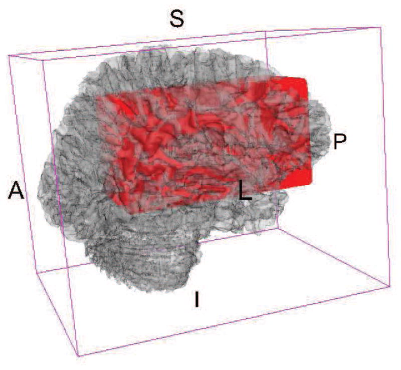
Red region contains the rectangular region we use as a predictor of cognitive function. Background 3D brain is rendered from a T1 template image.

Methods

The core of our approach is to assume that there is an underlying unknown 0/1 map of voxels indicating non-association or association with the outcome respectively, and place an Ising prior on this latent binary image. Our model can be implemented through a single-site Gibbs sampler, where the computation time needed for each sweep over the image space is linear in the number of locations and does not depend on the number of nonzero coefficients.

We first introduce some notation. Assume the data for subject i ∈ {1, 2, …, I} are {y_i, X_i, Z_i}, where y_i is the scalar outcome (e.g. cognitive score), X_i is a vectorized image of the ith subject, and Z_i consists of other covariates (e.g. gender, age, etc.). In the MS example, every image X_i is a 3-dimensional array structure of dimension L = L₁L₂L₃ = 61 · 125 · 26 = 198, 250, though in general it can be an arbitrary 3-D manifold. We represent X_i as an L×1 dimensional vector, (x_i1, x_i2, …, x_il, …, x_iL)^T, where x_il is an imaging measure, such as fractional anisotropy, for subject i at voxel location l.

Scalar-on-image regression: an ill-posed multiple linear regression

In essence, scalar-on-image regression is a multiple linear regression model, with the clinical outcome as the response and the image voxels as the predictors:

$$\begin{array}{l}{y}_i=\alpha +Z_i^T\eta +X_i^T\beta +{\epsilon }_i\\ =\alpha +Z_i^T\eta +\sum _{l=1}^L{x}_{il}{\beta }_l+{\epsilon }_i\end{array}$$ (1)

where β = (β₁, β₂, …, β_L)^T is a vector of coefficients for the image predictor X_i. In other words, each element β_l is the coefficient for the image intensity x_il at voxel l. The parameter β_l can be interpreted as the change in y_i for each unit change in x_il adjusting for all other locations (i.e., x_l′ for all l′ ≠ l). The errors ε_i are independent and identically distributed normal random variables with mean 0 and variance ${\sigma }_{\epsilon }^2$. See Figure 2 for an illustration.

Figure 2.

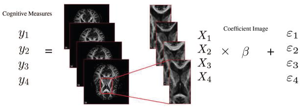
Illustration of the multiple linear regression model, with cognitive disability measure as the scalar response and fractional anisotropy maps as the image predictor.

When the intensities of all locations are mutually independent, solving this model will be equivalent to fitting separate linear regressions of y_i on x_il for each l. However, if the voxel-level measurements are correlated, this multiple linear regression can in principle provide improved estimation by incorporating information across the brain as a whole.

We note that, whereas most predictive or “decoding” methods in neuroimaging [Haynes and Rees, 2006; Norman et al., 2006] have focused on pattern classification, Equation (1) models continuous outcomes [Cohen et al., 2011]. The model can be extended to deal with classification problems, by assuming a discrete distribution for Y_i and using an appropriate generalized linear model.

Unfortunately, fitting the multiple linear regression model (1) is an ill-posed problem. The dimension of X (here X is the collection of images across subjects, i.e. X = (X₁, X₂, …, X_I)^T) is I × L and in most neuroimaging application I (the number of subjects) is much smaller than L (the number of voxels), so that the least-squares solution is not unique. In order to obtain an estimate of the coefficient, dimension-reducing assumptions are needed to narrow the solution space. Our algorithm, presented below, narrows the solution space to a set of coefficient maps which are sparse and spatially continuous.

Fitting through penalization and its connection to empirical Bayesian linear regression

A standard way to make the solution identifiable is the penalized regression, wherein the usual least-squares criterion minimized in linear regression is replaced by a penalized least squares criterion, i.e., the estimate for model (1) is given by

$$\widehat{\beta }={\mathit{argmin}}_{\beta \in {ℝ}^L}\left\{\sum _{i=1}^I{(y_i-\alpha -Z_i^T\eta -X_i^T\beta )}^2+P(\beta )\right\}.$$ (2)

The penalty P (β) is chosen to yield a solution to Equation (1) with desirable properties such as smoothness or sparsity.

Penalizing on β has a Bayesian interpretation: (2) is equivalent to enforcing a particular prior on the coefficients. Indeed, solving Equation (2) is statistically equivalent to the following model where the β coefficients are treated as random:

$$\{\begin{array}{c}{y}_i~N(\alpha +Z_i^T\eta +X_i^T\beta ,{\sigma }_{\epsilon }^2);\\ f(\beta )\propto exp\{-P^{-1}(\beta )/2\}.\end{array}$$ (3)

The solution β̂ of model (2) equals the posterior mean E(β|y) in Equation (3). The advantage of model (3) is that it provides a likelihood-based approach to fitting, which in turn allows inference on the model parameters. The second line of equation (3) means that β has a density function f(β) proportional to exp {−P⁻¹(β)/2}, where the normalizing constant is omitted. For specific forms of the penalty the prior distribution exp {−P⁻¹(β)/2} may be improper (i.e. its integral may not be finite). But as long as the posterior distribution of β|Y is proper, model (3) still provides reasonable results.

One of the most popular penalties is the ridge regression or ℓ₂ penalty [Hoerl and Kennard, 1970] P(β) = λβ^T β, where λ is a scalar tuning parameter, with λ = 0 corresponding to no penalty and λ = ∞ corresponding to β = 0. Using (3), it follows that a ridge penalty is equivalent to assuming that the β parameters have an independent multivariate normal prior with constant variance. The lasso or ℓ₁ penalty [Tibshirani, 1996; Park and Casella, 2008] P (β) = λΣ |β_l| is equivalent to an independent double exponential prior on β in (1). A similar connection holds for elastic net penalty [Zou and Hastie, 2005; Carroll et al., 2009; Ryali et al., 2010; de Brecht and Yamagishi, 2012], whose corresponding prior is a mixture of normal and double-exponential distribution.

Much recent work has been done to choose suitable spatial priors for neuroimaging data. For example, Penny et al. [2005] have proposed a fully Bayesian model with spatial priors defined over the regression coefficients of a general linear model, using Laplacian operators or a Gaussian Markov Random Field. Flandin and Penny [2007] have proposed a Bayesian approach using a sparse spatial basis function priors. This model allows for spatial variations in intensity smoothness. As an alternative, Everitt and Bullmore [1999]; Hartvig and Jensen [2000]; Woolrich and Behrens [2006] model the spatial distribution of activation maps using mixture models.

Connection with scalar-on-function regression

Equation (1) can be viewed as a discretized version of a functional linear regression model with scalar response. The functional regression model is written as

$$y_i=\alpha +Z_i^T\eta +\int X_i(t)\beta (t)dt+{\epsilon }_i,$$

where the integral is over a region of 3D Euclidean space. Ramsay and Silverman [2005] discuss models of this form for one-dimensional t, and many papers have been written on similar models for both continuous and categorical responses [James, 2002; Cardot et al., 2003; Müller and Stadtmüller, 2005; James and Silverman, 2005; Reiss and Ogden, 2007]. In equation (1), X_i is a discretization of X_i(t) on a three-dimensional lattice, which transforms the integral into a sum. In these scalar-on-function models, dimension reduction is achieved by imposing some structure on the coefficient function β(t)—for example, by assuming that it lies in the span of the leading functional principal components, and/or imposing a smooth estimate by means of penalized B-splines [Cardot et al., 2003; Müller and Stadtmüller, 2005; Reiss and Ogden, 2010]. However, it is unclear that such approaches would be effective and computationally feasible for multi-dimensional images containing tens or hundreds of thousands of voxels. In this setting it is natural to require the coefficient image to be both smooth and sparse. The prior that we describe next leads to estimates that meet these requirements.

Our proposal: Imposing an Ising prior on a latent 0/1 map

We are interested in priors ensuring that 1) neighboring voxels have similar coefficient values and 2) non-zero coefficients form contiguous patches in large areas of zero effects. Such local constraints are difficult to impose through ridge or lasso penalties, as they assume that the β parameters are exchangeable and do not incorporate spatial dependence. Thus, we focus on finding an appropriate prior distribution in the family of Markov random field spatial distributions. More precisely, we propose to use a neighborhood-based Ising prior [Cipra, 1987].

First, we introduce an L-dimensional binary random image γ such that β_l = 0 if γ_l = 0 and β_l ≠ 0 if γ_l = 1; the binary map γ is a map that indicates which locations in the image coefficient are zero and do not impact the outcome. One can view γ as an unknown brain mask that defines regions of interest. Here we are interested in estimating this mask. An Ising prior is used for γ, so that

$$p(\gamma )=\phi (a,b)exp\left[a\gamma +\sum _l\left\{\sum _{l^{\prime }\in {\delta }_l}bI({\gamma }_l={\gamma }_{l^{\prime }})\right\}\right]$$

where δ_l is the set of locations which are in the neighbourhood of location l and φ(a, b) is a normalizing constant. The parameters of the Ising distribution a and b control the overall sparsity and interaction between neighbouring points, respectively. Thus two assumptions are addressed: 1) sparsity controlled by a — most voxels have coefficient β_l = 0, which means there is no association with the measurement y_i; and 2) spatial contiguity controlled by b —a voxel is more likely to have a nonzero coefficient if its neighbours do. The parameters a and b could be allowed to vary spatially; for simplicity we assume that they are the same across locations.

Next, we assume that for those locations where the image is correlated with the outcome (i.e. γ_l = 1), β_l has a normal prior with an unknown variance ${\sigma }_{\beta }^2$. If ${\sigma }_{\beta }^2=+\infty$, then no shrinkage will be placed on the estimated β̂_l. We estimate ${\sigma }_{\beta }^2$ by cross-validation, and in practice have found that a small ${\sigma }_{\beta }^2$ achieves low prediction error in noisy data sets. More precisely $[{\beta }_l\mid {\gamma }_l=1,{\beta }_{-l}]~N(0,{\sigma }_{\beta }^2)$, which leads to the posterior conditional distribution

$$\begin{array}{c}[{\beta }_l\mid y,{\gamma }_l=1,{\beta }_{-l},\alpha ,\eta ]\propto [y\mid \beta ,{\gamma }_l=1,\alpha ,\eta ][{\beta }_l\mid {\gamma }_l,{\beta }_{-l}]\\ ~N[{\mu }_l,{\sigma }_l^2],\end{array}$$

where ${\mu }_l={\sigma }_l^2\left\{\frac{1}{{\sigma }_{\epsilon }^2}{(y-\alpha -Z^T\eta -X_{-l}^T{\beta }_{-l})}^T{x}_l\right\},{\sigma }_l^2={\left(\frac{1}{{\sigma }_{\epsilon }^2}{x}_l^T{x}_l+\frac{1}{{\sigma }_{\beta }^2}\right)}^{-1}$ are the location-specific posterior mean and variance. Following the above equations, the location-specific posterior distribution comparing (γ_l, β_l) = (0, 0) to (1, β^*) is $p\{({\gamma }_l=1,{\beta }_l={\beta }^{\ast })\mid y,{\beta }_{-l},{\gamma }_{-l}\}=\frac{1}{1+g}$ where

$$\begin{array}{l}g=\frac{p(y\mid {\beta }_l=0,{\beta }_{-l})p({\gamma }_l=0\mid {\gamma }_{-l})}{p(y\mid {\beta }_l={\beta }^{\ast },{\beta }_{-l})p({\beta }_l={\beta }^{\ast }\mid {\gamma }_l=1)p({\gamma }_l=1\mid {\gamma }_{-l})}\\ =exp[-\frac{1}{2{\sigma }_{\epsilon }^2}\{{(Y-\alpha -Z^T\eta -X^T{\beta }^0)}^T(Y-\alpha -Z^T\eta -X^T{\beta }^0)\\ -{(Y-\alpha -Z^T\eta -X^T{\beta }^1)}^T(Y-\alpha -Z^T\eta -X^T{\beta }^1)\}\\ +\frac{1}{2{\sigma }_l^2}{({\beta }^{\ast }-{\mu }_l)}^2-a+b\sum _{l^{\prime }\in {\delta }_l}\{I({\gamma }_l=0)-I({\gamma }_l=1)\}]\sqrt{2\pi {\sigma }_l^2}\end{array}$$

Here, β⁰ is the coefficient image corresponding to (γ_l, β_l) = (0, 0) while β¹ is the coefficient image corresponding to (γ_l, β_l) = (1, β^*), and β^* is sampled from the posterior distribution [β_l|y, γ_l = 1, β_−l, α, η].

Thus, at each image location the joint posterior distribution of the binary image and coefficient map is a Bernoulli choice that accounts for prior information through the Ising distribution as well as the relative impact of a zero and nonzero coefficient on the outcome likelihood.

Smith and Fahrmeir [2007] and Li and Zhang [2010] proposed similar Ising priors to select coefficients, but there are two important differences from our setting. Smith and Fahrmeir [2007] looked at a linear model at each voxel in an fMRI analysis. The Ising prior is placed across models. By contrast, we are placing Ising model on a single model and our aim is to predict an outcome from one single whole map. In both papers, the regression coefficients are calculated marginally. This method requires the inversion of matrix of size p × p, where p is the dimension of predictive coefficients. When p is large, this inversion is computationally infeasible. Instead, our method calculates the β_l by conditioning on other voxels during each sweep of the Gibbs sampler, which avoids the problem of large matrix inversion.

Advantages of the Ising prior

The Ising prior has some important properties that are useful for conducting computations. Most importantly, the Ising distribution admits the single-site conditional distribution $p({\gamma }_l=1\mid {\gamma }_{-l})=\frac{1}{1+g}$ where γ_−l is the vector of γ_l′ where l′ ≠ l and

$$g=\frac{p({\gamma }_l=0\mid {\gamma }_{-l})}{p({\gamma }_l=1\mid {\gamma }_{-l})}=exp\left[-a+b\sum _{l^{\prime }\in {\delta }_l}\{I({\gamma }_l=0)-I({\gamma }_l=1)\}\right].$$

This indicates that the probability for voxel l to be predictive knowing the status of all other voxels in the brain depends only on the status of the voxels in a defined neighborhood of the voxel (Here and below, we use “predictive” as shorthand for voxels with nonzero coefficients). This is intuitive and extremely helpful when one is interested in simulating from the posterior distribution of the latent 0/1 surface γ indicating whether a voxel is predictive or not. Indeed, instead of updating the entire image at once, one needs only update it one voxel at a time. This is why the algorithm is linear in the number of locations and remains relatively fast, even when the number of predictive locations is very large. Here we consider only contiguous, cubic neighbourhoods, though other definitions are also possible.

Estimation

Our full model is

$$\begin{array}{l}{y}_i~N(\alpha +Z_i^T\eta +X_i^T\beta ,{\sigma }_{\epsilon }^2)\\ {\beta }_l~\{\begin{array}{ll}\delta (0),\hfill & \text{if}{\gamma }_l=0\hfill \\ N\left[0,{\sigma }_{\beta }^2\right]\hfill & \text{if}{\gamma }_l=1\hfill \end{array}\\ {\gamma }_l~\text{Bernoulli}[p_l]\\ p_l~\text{Ising}[a,b]\end{array}$$

where δ(0) is a point-mass at zero. The Ising prior controls the number of nonzero coefficients and favors contiguity of localized effects. The Bernoulli choice between zero and nonzero coefficients at each location depends the posterior probability of whether a voxel is predictive or not. Goldsmith et al. [2013] used a similar model but imposed a conditional autoregressive (CAR) prior on β_l whose indicator variable γ_l equals 1 and used a much smaller number of predictor voxels (30K). Here we use an exchangeable prior on the size of effects at those locations that are found to be associated with the outcome.

We implement a single-site Gibbs sampler to generate iterates from the posterior distribution of (γ, β). At the tth step, we proceed through the following steps for each location l ∈ {1, 2, …, L}:

1. Calculate μ_l, ${\sigma }_l^2$ from ${\beta }_{-l}^{(t)}$

2. Generate ${\beta }_l^1~N({\mu }_l,{\sigma }_l^2)$

3. Calculate the posterior probability g from ${\beta }_{-l}^{(t)}$ and β¹

4. Generate ${\gamma }_l^{(t+1)}~\text{Bern}(g)$

5. If ${\gamma }_l^{(t+1)}=1,{\beta }_l^{(t+1)}={\beta }_l^1$; otherwise ${\beta }_l^{(t+1)}=0$.

Tuning parameters

The parameters a, b, ${\sigma }_{\epsilon }^2$ and ${\sigma }_{\beta }^2$ control the estimation of the coefficient map and are referred to as tuning parameters. Here ${\sigma }_{\epsilon }^2$ determines the impact of the change in the outcome likelihood on the overall probability whether a voxel is predictive or not. Similarly, in the posterior distribution of predictive regression coefficients, the parameter ${\sigma }_{\beta }^2$ is important in determining the posterior mean and variance. Finally, a controls the overall sparsity, while b determines the overall degree of smoothness among the γ parameters.

To select these tuning parameters we use five-fold cross validation. Our data are divided into five randomly selected groups. Each time, we obtain the training model from four groups and calculate the prediction error from the rest group. The procedure is repeated 5 times and the average of the prediction errors is calculated; the tuning parameter estimators (a, b, ${\sigma }_{\epsilon }^2,{\sigma }_{\beta }^2$) minimize this average prediction error. The choice of grid for tuning parameter is crucial – a grid range that is too narrow may miss the optimal parameters while a range that is too broad increases the computational burden. In the following simulation study, we provide some practical advices about the choice of the grid.

The model provides an excellent exploratory and sensitivity analysis tool where results can be inspected by simply changing the tuning parameters. We find this multi-resolution approach to be very helpful in the context where one is interested in further exploring results beyond simply using the cross validated values. Such an exploratory analysis could be based on modifications of the estimated tuning parameters.

An alternative is through a fully Bayesian model that imposes a hyperprior on the tuning parameters. Unfortunately, for the levels of signal-to-noise observed in brain imaging our fully Bayesian implementation was quite slow, strongly dependent on the prior on the Ising distribution parameters, and not particularly robust. Therefore, the full Bayesian model is feasible, but will require some non-trivial computational developments. For example, the posterior distributions of a and b are hard to obtain, and one must implement an empirical approximation to the normalizing constant to enable generation of a, b [Gelman and Meng, 1998].

Simulation

To further investigate the effect of choices of the tuning parameters as well as the performance of our method, we conducted a simulation study with two-dimensional predictors.

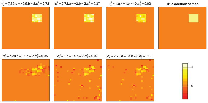
First, we generate the true coefficient map β on a 30×30 rectangle. All the coefficients are zero except that, in a 5×5 square, the coefficients are set to 1 (Figure 3). Then the predictors ( $X_i^S$) with the same dimension as the coefficient map are generated from a standard normal distribution. Simulated outcomes $y_i^S$ are given by $y_i^S=\alpha +X_i^S·\beta +{\epsilon }_i$ where α = 0 and ${\epsilon }_i~N(0,{\sigma }_{\epsilon }^2)$. We consider two levels for the variance ${\sigma }_{\epsilon }^2$: letting ${\sigma }_y^2=\text{Var}(X^S·\beta )$ be the sample variance of the simulated outcomes, we choose ${\sigma }_{\epsilon }^2$ such that the signal-to-noise ratio $\frac{{\sigma }_y^2}{{\sigma }_{\epsilon }^2}$ is either 1 or 10.

Figure 3.

Estimated coefficient maps separated by signal-to-noise ratios, choices of tuning parameters. The first row corresponds to the case when signal-to-noise ratio is 10 while the second row corresponds to the case when the ratio is 1. The first column shows the estimates when the optimal tuning parameters are used. For the second and third columns, we used two sets of randomly-picked tuning parameters whose CV score are at most 40% higher than the optimal value.

For each signal-to-noise ratio, we generate 499 datasets in the manner described above with I = 100 (number of the subjects). In the first dataset only we use five-fold cross validation to select the tuning parameters a, b, ${\sigma }_{\epsilon }^2,{\sigma }_{\beta }^2$. We then fix these tuning parameter values, we fit a scalar-on-image regression on each simulated dataset. On the one hand, because the tuning parameters are chosen based on the first simulated dataset, the results may not be fully representative of the proposed method. On the other hand, we can use this information to investigate the sensitivity of the model fits to possibly non-optimal tuning parameters. For each fit, the coefficient image β̂ is initialized to zero. We use 250 iterations of the Gibbs sampler and discard the first 100 as burn-in.

To evaluate the estimated coefficient images, we use the mean squared error (MSE) separately for regions in which β = 0 (“non-predictive”) and the remaining (“predictive”) regions, to provide insight into the method’s ability to accurately detect features while inducing sparsity elsewhere. Thus we define ${\text{MSE}}_1=\frac{1}{L_1}{\sum }_{l{\in }_{\text{predictive}}}{({\beta }_l-{\widehat{\beta }}_l)}^2$ and ${\text{MSE}}_0=\frac{1}{L_0}{\sum }_{l\in \text{non}-\text{predictive}}{({\beta }_l-{\widehat{\beta }}_l)}^2$ where L₁, L₀ are the numbers of predictive and non-predictive image locations. Table 1 displays the mean and standard deviation of both MSE components for each signal-to-noise ratio and its standard deviation.

Table 1.

Average mean square error separated by true predictive and non-predictive location, signal-to-noise ratios. In the brackets are the standard deviations of MSE across simulated datasets.

signal-to-noise ratio	MSE1	MSE0
10	1.602 × 10−1(3.444 × 10−2)	5.032 × 10−3(1.242 × 10−3)
1	6.662 × 10−1(8.485 × 10−2)	5.951 × 10−3(1.628 × 10−3)

For perspective on Table 1, in Figure 3 we display coefficient image estimates for simulations with the median MSE₁ scores. Although we used the tuning parameters from the first simulated data set rather than choosing them for each individual data set, the estimated coefficients are still reasonable, picking up the predictive region in the true coefficient map. Next, we fit the same simulated datasets again with other sets of tuning parameters whose CV scores are at most 40% higher than the optimal value. The estimated coefficients (the middle two columns of Figure 3) are worse than the optimal one (the first column of Figure 3), especially when the signal-to-noise ratio is low. However, the estimated coefficients still capture the key features of the true map.

As noted by a referee, using five-fold cross-validation to choose four tuning parameters is a hard problem. In practice, if one has some background knowledge about the data, it would help the choice. For example, Li and Zhang [2010] said if there is a priori belief in a sparse model, one can constrain the range of a, b in a small region. Or if the data is very noisy, one should choose a very small ${\sigma }_{\beta }^2$ as illustrated in our simulation study.

However, if there is no background knowledge, we employ a step-by-step procedure. We start with a sparse grid in a broad range and gradually refine the grid at each iteration. For example, in this simulation study, we first looked at the grid of tuning parameters in the log scale, i.e. ${\sigma }_{\epsilon }^2,{\sigma }_{\beta }^2$,b are selected from exp(−5) to exp(3) and a is selected from −exp(−5) to −exp(3). If the CV-optimizing tuning parameters lie on the boundary of the grid, we extend the grid and repeat the above cross validation. We then take out a 3 × 3 × 3 × 3 sub-grid of which the set of tuning parameters with the optimal CV score is in the middle. Last, we refine the above sub-grid into a 7 ×7 ×7 ×7 grid using the natural scale, with boundary and the middle point unchanged. In the end, the optimal tuning parameters are obtained based on the cross-validation.

DTI study

As discussed in the Introduction, our motivating application is to investigate the relationship between cognitive disability in MS patients and their diffusion tensor images. MS is an immune-mediated disease that affects the brain and spinal cord (central nervous system). It results in damage to the myelin sheath, the protective covering that surrounds axons in white matter. Damage caused by MS can disrupt the transmission of signals in affected tracts.

Study participants with MS were recruited from an outpatient neurology clinic and healthy volunteers from the community. All disability scores were measured within 30 days of the MRI scan. Prior to MRI scanning and disability testing, all participants gave signed, informed consent. All procedures were approved by the institutional review board, and previous results on this dataset have been reported [Goldsmith et al., 2011; Reich et al., 2010; Ozturk et al., 2010].

We used the Paced Auditory Serial Addition Test (PASAT) as a proxy measurement for cognitive disability. This score assesses mental capacity, rate of information processing, and sustained and divided attention. The range of PASAT is from 0 to 60, with higher scores indicating better cognition ability [Fischer et al., 1999].

All DTI scans were performed on a 3T scanner (Intera; Philips, Best, The Netherlands) over a 4.6 year period, using the body coil for transmission and either a 6-channel head coil or the 8 head elements of a 16-channel neurovascular coil for reception (both coils are made by Philips). Each session included two sequential DTI scans using a conventional spin-echo sequence and a single-shot EPI readout. Whole-brain data were acquired in nominal 2.2 mm isotropic voxels and with the following parameters: TE, 69 ms; TR, automatically calculated (“shortest”); slices, 60 or 70; parallel imaging factor, 2.5; non-collinear diffusion directions, 32 (Philips “overplus high” scheme); high b-value, 700 s/mm²; low b-value (“b₀”), approximately 33 s/mm²; repetitions, 2; reconstructed in-plane resolution, 0.82 × 0.82 mm. We coregistered the diffusion-weighted scans to the minimally diffusion-weighted scan from the first DTI sequence using a rigid-body transformation implemented in the Automatic Image Registration program [Woods et al., 1998]. Prior to further analysis, data were adjusted to account for changes in average tract-specific MRI indices that resulted from scanner upgrades, by a procedure previously described by Harrison et al. [2011].

Here we focus on fractional anisotropy (FA) [Cercignani et al., 2001; Hasan et al., 2005]. The diffusion-weighted scans were processed using CATNAP [Landman et al., 2007] to create maps of FA. The whole-brain FAs were calculated by slice-wise averaging of all diffusion-weighted images, removal of the low-intensity voxels that are characteristic of extracerebral tissues on these images, and final removal of voxels with MD > 1.7 μm²/ms to exclude cerebrospinal fluid [Ozturk et al., 2010]. The resulting brain mask was applied to all DTI maps.

In summary, our study consists of data from 135 MS patients. Each has one PASAT score and one FA image with dimension 61 × 125 × 26, registered to ensure major structures (e.g., the corpus callosum) are aligned across subjects.

Results

After choosing the tuning parameters a, b, ${\sigma }_{\epsilon }^2,{\sigma }_{\beta }^2$ by cross-validation, we run the image regression model through the Gibbs sampling algorithm. We use a chain of length 500 and discard the first 100 samples as burn-in. All the regression coefficients and latent binary indicators are initialized at 0.

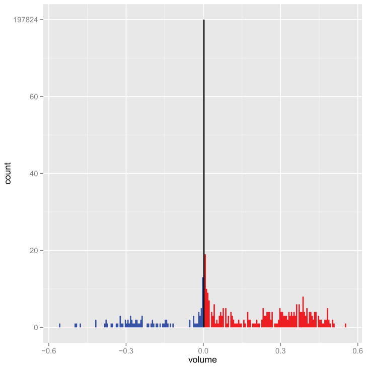
Figure 4 shows the overall distribution of estimated regression coefficients in β, and Figure 5 shows the estimated coefficients overlaid on an anatomical reference from Slice 7 to Slice 22. The first thing to notice is that most of coefficients are zero (426 of the 197842 voxels had β_l ≠ 0), due to the sparsity-inducing effect of the Ising prior. Figure 4 indicates that the number of coefficients with positive coefficient estimates (red lines) is larger than the number of negative estimates (blue lines). Thus, in most of the predictive voxels, lower FA values correspond to lower PASAT scores. This agrees with the scientific hypothesis that degradation of white matter is associated with diminished cognitive ability. Moreover, in Figure 5 the “visible” predictive regions, though extremely sparse, are located in the corpus callosum — the largest white matter structure in the brain, which has been related to cognitive ability [Ozturk et al., 2010] rather than nearby structures such as the internal capsule and thalamus.

Figure 4.

Histogram of the estimated coefficients with tuning parameter values a = −3, b = 6, ${\sigma }_{\epsilon }^2=1.22,{\sigma }_{\beta }^2=0.05$, which were chosen by five-fold cross-validation. The middle bar refers to coefficients whose magnitude is exactly 0. The blue bars denote the coefficients which are less than 0 while the red ones denote the coefficients that are positive.

Figure 5.

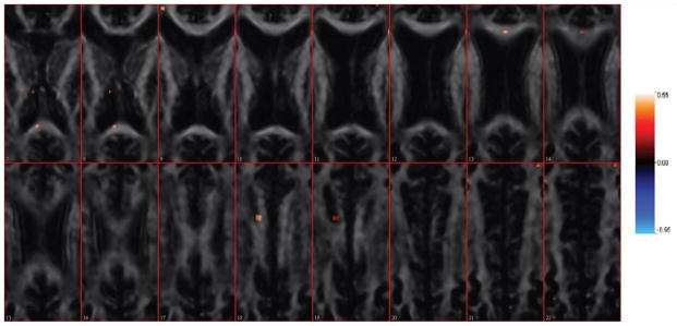
The estimated coefficient images from Slice 7 to Slice 22. The estimation is overlaid on one single subject’s FA scan image for anatomical reference. The tuning parameters are selected via cross validation, a = −3, b = 6, ${\sigma }_{\epsilon }^2=1.22,{\sigma }_{\beta }^2=0.05$. Positive coefficients are shown in red, while blue denotes negative coefficients. The estimated mean square prediction error is 146.43 and the proportion of variance explained for predicted data is 22.00%.

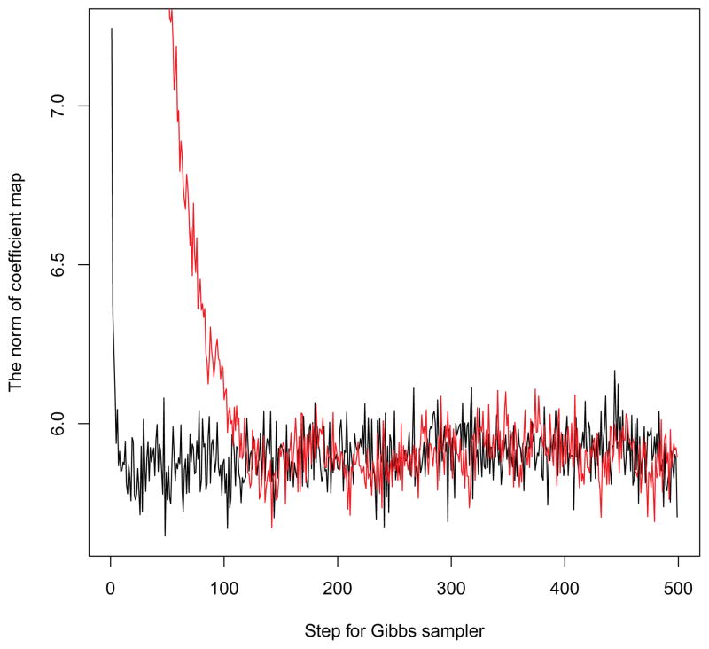
In Figure 6, we investigate the mixing and convergence properties of our Gibbs sampler. The coefficient map has a dimension equal to the number of voxels, and we use the norm of the coefficients (i.e. ${\left({\displaystyle \sum _{l=1}^L}{\beta }_l^2\right)}^{1/2}$) to illustrate the performance of the chain. The black line used the initial value 0, which is implemented in this paper. It converges very quickly, far before the end of the burn-in period. The red line is using the random generated initial value. It began to converge around step 150. We also compared two posterior means of the estimated coefficient images, and there is no major disparities of the results. Therefore both chains appear to converge to the same distribution.

Figure 6.

The chain of the norm of coefficient map from step 2 to step 500 of the Gibbs sampler. The black line gives the result when the initial values for coefficients are zero. The red line gives the result when the initial values are generated from a Normal(0,1) distribution.

Up to this point, we have used cross-validation to select tuning parameters and have provided estimated coefficient images that satisfy the sparsity and spatial continuity assumptions. However, one might be interested in exploring results as one moves away from the optimal cross-validated values of parameters. In fact, only 426 out of 198,250 voxels have nonzero coefficients, probably because data are noisy and cross validation heavily penalizes coefficients. This helps prediction but may be too restrictive when one is interested in exploratory data analysis and hypothesis generation. For exploratory purposes, one may be interested in obtaining less conservative coefficient images.

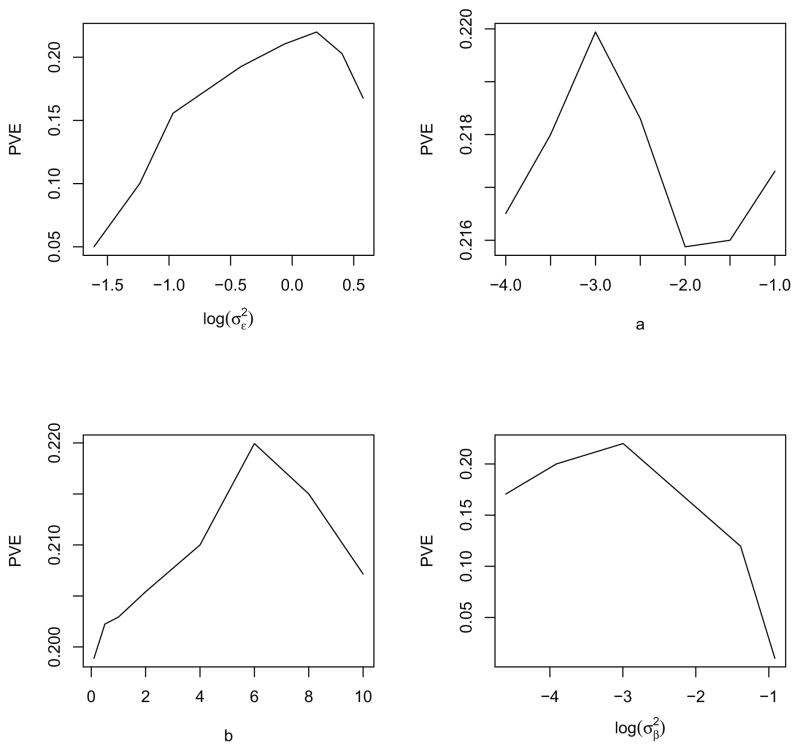
To guide an exploratory consideration of alternative tuning parameter values, the profile cross-validation plots (Figure 7) can provide insight into the effect of each tuning parameter on the performance of the model. In each of the four panels, three of the tuning parameters are fixed at the optimal values chosen by cross-validation, while the remaining tuning parameter varies in the x-axis. As shown in the figure, tuning parameters a, b have relatively small influence on the prediction performance. Thus, the empirical choice of those two parameters can be more flexible. Also, as ${\sigma }_{\beta }^2$ increases, the proportion of variance explained in left-out data drops dramatically, which indicates the shrinkage of β’s is necessary.

Figure 7.

Profile cross validation plot: in each panels three of the tuning parameters are fixed at the values chosen by cross-validation while the remaining tuning parameter varies in the x-axis. The y-axis is the proportion of variance explained in the left-out data.

Figures 8 and 9 present the coefficient images that result from two combinations of tuning parameters. Starting from the cross-validation setting (Figure 5), we select the tuning parameters (i.e. increase a, decrease b, decrease ${\sigma }_{\beta }^2$ and decrease ${\sigma }_{\epsilon }^2$) so that the estimation becomes less conservative. While a higher number of predictive regions are revealed from Figure 8 and Figure 9, the prediction power of the corresponding models is decreased. Table 3 shows the estimated mean of squared prediction errors and the proportion of variance explained for predicted data corresponding to Figures 5, 8 and 9. From this we can see that a range of coefficient images can provide similar results in terms of prediction power, and the choice of final model depends on both prediction accuracy and interpretation of the estimated coefficient image.

Figure 8.

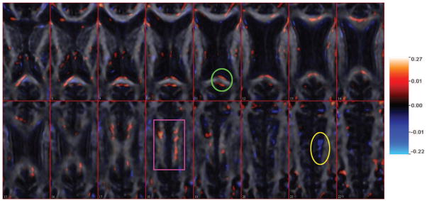
The estimated coefficient images from Slice 7 to Slice 22 using tuning parameters a = −2, b = 0.5, ${\sigma }_{\epsilon }^2=1,{\sigma }_{\beta }^2=0.03$. The estimation is overlaid on one single subject’s FA scan image for anatomical reference. The estimated mean square prediction error is 150.25 and the proportion of variance explained for predicted data is 20.34%.

Figure 9.

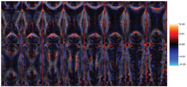
The estimated coefficient images from Slice 7 to Slice 22 using tuning parameters a = −1, b = 0.5, ${\sigma }_{\epsilon }^2=0.775,{\sigma }_{\beta }^2=0.05$. The estimation is overlaid on one single subject’s FA scan image for anatomical reference. The estimated mean square prediction error is 164.6 and the proportion of variance explained for predicted data is 19.22%.

Table 3.

Prediction performance of the tuning parameter combinations for Figures 5, 8, 9. The last two columns refer to mean square prediction error and proportion of variance explained.

Figure	${\sigma }_{\epsilon }^2$	a	b	${\sigma }_{\beta }^2$	MSE	PVE
5	1.22	−3	6	0.05	146.43054	0.22000
8	1	−2	0.5	0.03	150.25746	0.20341
9	0.775	−1	0.5	0.05	164.60563	0.19220

Balancing between prediction accuracy and result interpretation, in Figure 8, we choose a = −2, b = 0.5, ${\sigma }_{\epsilon }^2=1,{\sigma }_{\beta }^2=0.03$. In the estimated coefficient image, 41455 out of 198250 voxels have nonzero coefficients. Although significant effects tend to be located in the upper-left region comparing to a scattered pattern in the right side (e.g. marked with a purple rectangle), the coefficients on both sides maintain spatial contiguity. Most positive coefficients are located in the corpus callosum, which indicates that cognitive ability may be positively associated with integrity of the white matter in that region. We also found negative coefficients outside corpus callosum (e.g., in the lower-right region of Slice 21 marked with a yellow circle). This might be due to the undersmoothed estimation caused by a small b value, though further investigation is necessary. Several predictive regions (marked with a green circle) are located on the edge of the white matter, possibly due to registration error.

As noted by a referee, it can be difficult to understand the effect of tuning the four parameters on the estimated coefficient image. In practice we recommend using only the CV-optimizing tuning parameter values to form a final estimate, while noting that this method (like any method for regression with dimension far exceeding the sample size) is inherently exploratory. It may be useful to consider other tuning parameter values as a sensitivity analysis. In particular we recommend focusing only on tuning a, b. Both of these parameters have clear interpretations — controlling sparsity and heterogeneity of neighbourhood voxels, respectively — which makes easier to understand the effect of empirical tuning on the coefficient estimates.

For comparison, we first performed voxel-wise regressions, with PASAT score regressed on the FA values for each voxel in 198,250 separate linear regressions. (Note that in standard mass-univariate regression, the roles of PASAT and FA would be reversed.) In Figure 10, we plot the uncorrected p-values of the slope coefficients from Slice 7 to Slice 22. Most voxels with small p-values are located in the corpus callosum, as expected. Moreover, the regions with small p-values in the voxel-wise regressions tend to have large coefficients in our scalar-on-image regression.

Figure 10.

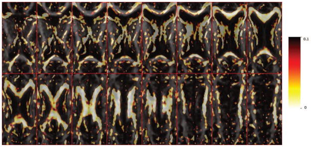
p-value map for voxel-wise linear regression fitting from Slice 7 to Slice 22.

Comparing the results in Figure 8 with Figure 10, the voxels with small p-values in Figure 10 spread symmetrically to the left and right part of the brain while our method shows an asymmetric pattern of predictive coefficients. For example, in Slice 18 there are predictive coefficients located in the upper-left region while in the right part, the significant coefficients are more evenly distributed across the corpus callosum (marked with purple rectangle). This difference is due to the fact that the scalar-on-image regression model fits the entire brain region at the same time. It estimates the effect of one voxel, adjusting for associations at other voxels. The voxelwise regressions do not have such adjustment.

For comparison with a method that is not spatially informed, we performed lasso regression on the same brain region, with the optimal shrinking parameter chosen by five-fold cross validation. The resulting MSE is 157.12, somewhat higher than the value for our proposed algorithm in Table 3. Due to the low signal-to-noise ratio, the lasso estimate is very conservative. Only 33 voxels are estimated to have non-zero coefficients, which are displayed in Figure 11. Most of the predictive voxels from lasso regression also appear in Figure 5. However, since there is no spatial constraint for the coefficients, those predictive voxels are scattered and do not form clusters (Figure 11).

Figure 11.

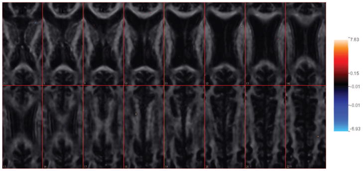
Coefficient map for the linear lasso regression fitting from Slice 7 to Slice 22.

An alternative non-spatially-informed method is to prescreen the voxels based on the standardized coefficients (i.e. β_l/σ_l) from separate voxelwise regressions, and then perform linear ridge regression using the selected voxels. In this study, we investigated 10, 100, 1000, 10000 voxels with the largest absolute standardized coefficients. The tuning parameters in the ridge regressions are selected by 5-fold cross validation and the estimated MSEs are 128.91, 107.92, 106.91, 101.00. The coefficient images for the top 100 and top 1000 voxels are presented in Figure 12. Since there is no spatial structure incorporated in the screening stage and regression stage, comparing to Figure 5, we can see two voxels with different signs in the adjacent voxels in Figure 12. Moreover, in the case of top 1000 voxels, we can identify some clear negative coefficients along the white matter in slice 18, which may not be scientifically meaningful [Ozturk et al., 2010]. However, this method does have a better prediction performance than either our proposed method or lasso regression. This indicates that the screening stage helps prediction performance. In future work, it may be worthwhile to incorporate a prescreening step, which does not ignore the spatial structure in the image, into our proposed method.

Figure 12.

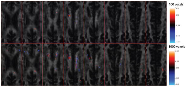
Coefficient map for the linear ridge regressions using top 100 and top 1000 voxel predictors. Slice 15 to Slice 22 are presented.

Discussion

We have proposed a novel linear regression approach for analyzing the relationship between cognitive disability and white matter microstructure in three-dimensional images. Noting the connection between penalized linear regression and Bayesian modeling, we proposed a Bayesian regression model with a latent binary indicator. We take advantage of an Ising prior to impose the assumption of sparsity and spatial continuity in the analysis. A distinctive merit of our method is that the regression model can be established on any manifold. By contrast, most scalar-on-image regression approaches [e.g. Reiss and Ogden, 2010; Reiss et al., 2013] require a regular grid. For simplicity, in our application we focused on a rectangular region, but the method is easy to extend to any irregularly shaped region, including the entire brain.

We applied our model to a multiple sclerosis study. The results show most of the predictive regions are located at the corpus callosum, as expected from existing work, not just in MS [Kern et al., 2010; Lin et al., 2008, 2005; Lowe et al., 2006; Ozturk et al., 2010] but in other diseases, including autism [Barnea-Goraly et al., 2004; Keller et al., 2007]. The corpus callosum connects the two cerebral hemispheres and thus mediates functions that require integration across multiple brain regions. Reflecting the overall increase in white matter in higher mammals, its thickness is substantially greater in humans than in rodents. Thus, it is not surprising that it plays a role in cognitive function, and that damage to the corpus callosum is associated with cognitive dysfunction in disease states. In interpreting the maps of Figures 5, 8 and 9, it is important to keep in mind that MS is a disease that affects the whole brain, not just the corpus callosum, and that the salient pathologies are perivenular inflammation and demyelination with axonal transections. At the same time, MS can also affect the brain in a tract-specific manner through processes such as Wallerian degeneration and dying-back axonopathy, which involve proximal and distal degeneration related to axonal transection anywhere along a fiber bundle. For these reasons, damage to portions of the corpus callosum that mediate cognition is very likely to be coupled to damage to nearby portions with other functions. It is therefore not surprising to us that the nonzero voxels identified by our method are distributed in space across our region of interest. It would be interesting to further develop these results by examining whether the specific voxels identified are spatially related to areas of focal white matter damage in this population, and whether, in other more homogeneous diseases, the voxels uncovered by the analysis are more localized in space. One example might be the so-called reversible splenium lesion [Takanashi et al., 2006].

There are a few limitations in the presented methodology. 1) If we choose the hyper-parameters via cross-validation, the computation time is high; this can be partially alleviated by parallel computing. Alternatively, a pilot cross-validation study can be done on part of the image region and the estimated parameters can then be applied to the entire image. 2) In addition to computation considerations, special attention must be paid to the stability of the results as both cross-validation and the Gibbs sampler are inherently stochastic methods. To examine this issue, we repeated cross-validation and cross validation distributions of tuning parameters are now plotted in Figure 13. From these plots we conclude that there is sizeable variability in both the a and b parameter estimates (the upper right and the lower left panels), which agrees with our profile cross validation plots. 3) Our approach is a hybrid between a Bayesian and a frequentist approach, where the hyper-parameter and coefficient estimation proceeds in parallel. A fully Bayesian approach might provide a more integrated and philosophically satisfying alternative. 4) We emphasize the sparsity of the coefficient image. In some analyses, one may be interested in borrowing strength from the immediate neighbours, as done via the CAR prior in Goldsmith et al. [2013]. Also, our current model only incorporates the neighbourhood information and emphasize on the sparsity of the predictive regions. We can also consider putting extra constraints on the coefficients to force the regions in white matter to have higher probabilities to be predictive. 5) We note that our method, when applied to FA maps, does not take registration error into account. Concerns about registration have motivated the development of tract-based analyses for DTI data [Smith et al., 2006]. Zhu et al. [2010, 2011] developed a functional linear model framework approach to tract-based data in which the DTI-derived functions are treated as the responses, unlike our method which uses the image data as the predictors.

Figure 13.

Histograms for each selected tuning parameters in 10 repeats of 5-fold cross validation. The upper left panel is for ${\sigma }_{\epsilon }^2$, the upper right panel is for a, the lower left is for b and the lower right is for ${\sigma }_{\beta }^2$.

Avenues for further work include the following. (1) Instead of a continuous response variable, we can extend our model to cope with categorical variable for classification problems. A Metropolis-Hastings algorithm will be implemented to sample from the conditional posterior distribution during Gibbs sampling. (2) We will develop inferential tools for statistical testing for image regression. As an analogy to the confidence band in frequentist inference [Reiss and Ogden, 2010], we can construct credible interval (or Bayesian posterior interval) from the Gibbs samples. (3) In terms of application, we may consider extending the analysis to the entire brain or to using other imaging-based measurements within our current region of interest. It is also fairly straightforward to extend our method to single-subject fMRI data. For multiple-subject fMRI data, one possible solution is to incorporate a spatio-temporal process into the prior of the scalar-on-image regression model [Woolrich et al., 2004].

Table 2.

MS patient characteristics. Disability data were obtained within 30 days of the MRI scan.

No. of participants (% women)	135 (35%)
Mean age, years (SD; range)	44 (12; 20–69)
Mean PASAT (SD; max=60)	44 (13)

Highlights.

• We analyze the relationship between cognitive outcomes and DTI predictors.

• We jointly model the predictive status and the regression coefficient.

• We induce the sparsity and promote spatial continuity in the model.

• The model is esimated through a Gibbs sampler, which is computational efficient.

• The model can be carried out over a large and irregular brain region.

References

- Ashburner J, Friston KJ. Voxel-based morphometry—the methods. NeuroImage. 2000;11:805–821. doi: 10.1006/nimg.2000.0582. [DOI] [PubMed] [Google Scholar]
- Barkhof F. The clinico-radiological paradox in multiple sclerosis revisited. Current Opinion in Neurology. 2002;15:239. doi: 10.1097/00019052-200206000-00003. [DOI] [PubMed] [Google Scholar]
- Barnea-Goraly N, Kwon H, Menon V, Eliez S, Lotspeich L, Reiss AL. White matter structure in autism: preliminary evidence from diffusion tensor imaging. Biological Psychiatry. 2004;55:323–326. doi: 10.1016/j.biopsych.2003.10.022. [DOI] [PubMed] [Google Scholar]
- de Brecht M, Yamagishi N. Combining sparseness and smoothness improves classification accuracy and interpretability. NeuroImage. 2012;60:1550–1561. doi: 10.1016/j.neuroimage.2011.12.085. [DOI] [PubMed] [Google Scholar]
- Cardot H, Ferraty F, Sarda P. Spline estimators for the functional linear model. Statistica Sinica. 2003;13:571–592. [Google Scholar]
- Carroll MK, Cecchi GA, Rish I, Garg R, Rao AR. Prediction and interpretation of distributed neural activity with sparse models. NeuroImage. 2009;44:112–122. doi: 10.1016/j.neuroimage.2008.08.020. [DOI] [PubMed] [Google Scholar]
- Cercignani M, Inglese M, Pagani E, Comi G, Filippi M. Mean diffusivity and fractional anisotropy histograms of patients with multiple sclerosis. American Journal of Neuroradiology. 2001;22:952–958. [PMC free article] [PubMed] [Google Scholar]
- Ciccarelli O, Catani M, Johansen-Berg H, Clark C, Thompson A. Diffusion-based tractography in neurological disorders: concepts, applications, and future developments. The Lancet Neurology. 2008;7:715–727. doi: 10.1016/S1474-4422(08)70163-7. [DOI] [PubMed] [Google Scholar]
- Cipra BA. An introduction to the Ising model. American Mathematical Monthly. 1987;94:937–959. [Google Scholar]
- Cohen JR, Asarnow RF, Sabb FW, Bilder RM, Bookheimer SY, Knowlton BJ, Poldrack RA. Decoding continuous variables from neuroimaging data: basic and clinical applications. Frontiers in Neuroscience. 2011:5. doi: 10.3389/fnins.2011.00075. [DOI] [PMC free article] [PubMed] [Google Scholar]
- Efron B. Empirical Bayes estimates for large-scale prediction problems. Journal of the American Statistical Association. 2009;104:1015–1028. doi: 10.1198/jasa.2009.tm08523. [DOI] [PMC free article] [PubMed] [Google Scholar]
- Everitt BS, Bullmore ET. Mixture model mapping of brain activation in functional magnetic resonance images. Human Brain Mapping. 1999;7:1–14. doi: 10.1002/(SICI)1097-0193(1999)7:1<1::AID-HBM1>3.0.CO;2-H. [DOI] [PMC free article] [PubMed] [Google Scholar]
- Fischer JS, Rudick RA, Cutter GR, Reingold SC, Reingold The Multiple Sclerosis Functional Composite measure (MSFC): an integrated approach to MS clinical outcome assessment. Multiple Sclerosis. 1999;5:244–250. doi: 10.1177/135245859900500409. [DOI] [PubMed] [Google Scholar]
- Flandin G, Penny WD. Bayesian fMRI data analysis with sparse spatial basis function priors. NeuroImage. 2007;34:1108–1125. doi: 10.1016/j.neuroimage.2006.10.005. [DOI] [PubMed] [Google Scholar]
- Friston KJ, Holmes AP, Worsley KJ, Poline JP, Frith CD, Frackowiak RSJ. Statistical parametric maps in functional imaging: a general linear approach. Human Brain Mapping. 1994;2:189–210. [Google Scholar]
- Gelman A, Meng XL. Simulating normalizing constants: From importance sampling to bridge sampling to path sampling. Statistical Science. 1998:163–185. [Google Scholar]
- Goldsmith J, Crainiceanu CM, Caffo BS, Reich DS. Penalized functional regression analysis of white-matter tract profiles in multiple sclerosis. NeuroImage. 2011;57:431–439. doi: 10.1016/j.neuroimage.2011.04.044. [DOI] [PMC free article] [PubMed] [Google Scholar]
- Goldsmith J, Huang L, Crainiceanu CM. Smooth scalar-on-image regression via spatial bayesian variable selection. Journal of Computational and Graphical Statistics. 2013 doi: 10.1080/10618600.2012.743437. to appear. [DOI] [PMC free article] [PubMed] [Google Scholar]
- Goodin DS. Magnetic resonance imaging as a surrogate outcome measure of disability in multiple sclerosis: have we been overly harsh in our assessment? Annals of Neurology. 2006;59:597–605. doi: 10.1002/ana.20832. [DOI] [PubMed] [Google Scholar]
- Harrison DM, Caffo BS, Shiee N, Farrell JAD, Bazin PL, Farrell SK, Ratchford JN, Calabresi PA, Reich DS. Longitudinal changes in diffusion tensor–based quantitative MRI in multiple sclerosis. Neurology. 2011;76:179–186. doi: 10.1212/WNL.0b013e318206ca61. [DOI] [PMC free article] [PubMed] [Google Scholar]
- Hartvig NV, Jensen JL. Spatial mixture modeling of fMRI data. Human Brain Mapping. 2000;11:233–248. doi: 10.1002/1097-0193(200012)11:4<233::AID-HBM10>3.0.CO;2-F. [DOI] [PMC free article] [PubMed] [Google Scholar]
- Hasan KM, Gupta RK, Santos RM, Wolinsky JS, Narayana PA. Diffusion tensor fractional anisotropy of the normal-appearing seven segments of the corpus callosum in healthy adults and relapsing-remitting multiple sclerosis patients. Journal of Magnetic Resonance Imaging. 2005;21:735–743. doi: 10.1002/jmri.20296. [DOI] [PubMed] [Google Scholar]
- Haxby JV, Gobbini MI, Furey ML, Ishai A, Schouten JL, Pietrini P. Distributed and overlapping representations of faces and objects in ventral temporal cortex. Science. 2001;293:2425–2430. doi: 10.1126/science.1063736. [DOI] [PubMed] [Google Scholar]
- Haynes JD, Rees G. Decoding mental states from brain activity in humans. Nature Reviews Neuroscience. 2006;7:523–534. doi: 10.1038/nrn1931. [DOI] [PubMed] [Google Scholar]
- Hoerl AE, Kennard RW. Ridge regression: Biased estimation for nonorthogonal problems. Technometrics. 1970;12:55–67. [Google Scholar]
- James GM. Generalized linear models with functional predictors. Journal of the Royal Statistical Society: Series B. 2002;64:411–432. [Google Scholar]
- James GM, Silverman BW. Functional adaptive model estimation. Journal of the American Statistical Association. 2005;100:565–576. [Google Scholar]
- Keller TA, Kana RK, Just MA. A developmental study of the structural integrity of white matter in autism. Neuroreport. 2007;18:23–27. doi: 10.1097/01.wnr.0000239965.21685.99. [DOI] [PubMed] [Google Scholar]
- Kern KC, Sarcona J, Montag M, Giesser BS, Sicotte NL. Corpus callosal diffusivity predicts motor impairment in relapsing-remitting multiple sclerosis: A TBSS and tractography study. NeuroImage. 2010;55:1699–1677. doi: 10.1016/j.neuroimage.2010.10.077. [DOI] [PubMed] [Google Scholar]
- Landman BA, Farrell JAD, Jones CK, Smith SA, Prince JL, Mori S. Effects of diffusion weighting schemes on the reproducibility of DTI-derived fractional anisotropy, mean diffusivity, and principal eigenvector measurements at 1.5 T. NeuroImage. 2007;36:1123–1138. doi: 10.1016/j.neuroimage.2007.02.056. [DOI] [PubMed] [Google Scholar]
- Li F, Zhang NR. Bayesian variable selection in structured high-dimensional covariate spaces with applications in genomics. Journal of the American Statistical Association. 2010;105:1202–1214. [Google Scholar]
- Lin X, Tench CR, Morgan PS, Constantinescu CS. Use of combined conventional and quantitative MRI to quantify pathology related to cognitive impairment in multiple sclerosis. Journal of Neurology, Neurosurgery & Psychiatry. 2008;79:437–441. doi: 10.1136/jnnp.2006.112177. [DOI] [PubMed] [Google Scholar]
- Lin X, Tench CR, Morgan PS, Niepel G, Constantinescu CS. ‘Importance sampling’ in MS: Use of diffusion tensor tractography to quantify pathology related to specific impairment. Journal of the Neurological Sciences. 2005;237:13–19. doi: 10.1016/j.jns.2005.04.019. [DOI] [PubMed] [Google Scholar]
- Lowe MJ, Horenstein C, Hirsch JG, Marrie RA, Stone L, Bhattacharyya PK, Gass A, Phillips MD. Functional pathway-defined MRI diffusion measures reveal increased transverse diffusivity of water in multiple sclerosis. NeuroImage. 2006;32:1127–1133. doi: 10.1016/j.neuroimage.2006.04.208. [DOI] [PubMed] [Google Scholar]
- Müller HG, Stadtmüller U. Generalized functional linear models. Annals of Statistics. 2005;33:774–805. [Google Scholar]
- Norman KA, Polyn SM, Detre GJ, Haxby JV. Beyond mind-reading: multi-voxel pattern analysis of fMRI data. Trends in Cognitive Sciences. 2006;10:424–430. doi: 10.1016/j.tics.2006.07.005. [DOI] [PubMed] [Google Scholar]
- Ozturk A, Smith SA, Gordon-Lipkin EM, Harrison DM, Shiee N, Pham DL, Caffo BS, Calabresi PA, Reich DS. MRI of the corpus callosum in multiple sclerosis: association with disability. Multiple Sclerosis. 2010;16:166–177. doi: 10.1177/1352458509353649. [DOI] [PMC free article] [PubMed] [Google Scholar]
- Park T, Casella G. The Bayesian Lasso. Journal of the American Statistical Association. 2008;103:681–686. [Google Scholar]
- Penny WD, Trujillo-Barreto NJ, Friston KJ. Bayesian fMRI time series analysis with spatial priors. NeuroImage. 2005;24:350–362. doi: 10.1016/j.neuroimage.2004.08.034. [DOI] [PubMed] [Google Scholar]
- Purcell SM, Wray NR, Stone JL, Visscher PM, O’Donovan MC, Sullivan PF, Sklar P, Ruderfer DM, McQuillin A, Morris DW, et al. Common polygenic variation contributes to risk of schizophrenia and bipolar disorder. Nature. 2009;460:748–752. doi: 10.1038/nature08185. [DOI] [PMC free article] [PubMed] [Google Scholar]
- Ramsay JO, Silverman BW. Functional Data Analysis. 2 New York: Springer; 2005. [Google Scholar]
- Reich DS, Ozturk A, Calabresi PA, Mori S. Automated vs. conventional tractography in multiple sclerosis: Variability and correlation with disability. NeuroImage. 2010;49:3047–3056. doi: 10.1016/j.neuroimage.2009.11.043. [DOI] [PMC free article] [PubMed] [Google Scholar]
- Reiss PT, Huo L, Ogden RT, Zhao Y, Kelly C. Wavelet-domain scalar-on-image regression, with an application to psychiatric diagnosis. 2013 Under revision. Available at http://works.bepress.com/phil_reiss/29/
- Reiss PT, Mennes M, Petkova E, Huang L, Hoptman MJ, Biswal BB, Colcombe SJ, Zuo XN, Milham MP. Extracting information from functional connectivity maps via function-on-scalar regression. NeuroImage. 2011;56:140–148. doi: 10.1016/j.neuroimage.2011.01.071. [DOI] [PMC free article] [PubMed] [Google Scholar]
- Reiss PT, Ogden RT. Functional principal component regression and functional partial least squares. Journal of the American Statistical Association. 2007;102:984–996. [Google Scholar]
- Reiss PT, Ogden RT. Functional generalized linear models with images as predictors. Biometrics. 2010;66:61–69. doi: 10.1111/j.1541-0420.2009.01233.x. [DOI] [PubMed] [Google Scholar]
- Ryali S, Supekar K, Abrams DA, Menon V. Sparse logistic regression for whole brain classification of fMRI data. NeuroImage. 2010;51:752. doi: 10.1016/j.neuroimage.2010.02.040. [DOI] [PMC free article] [PubMed] [Google Scholar]
- Smith M, Fahrmeir L. Spatial bayesian variable selection with application to functional magnetic resonance imaging. Journal of the American Statistical Association. 2007;102:417–431. [Google Scholar]
- Smith SM, Jenkinson M, Johansen-Berg H, Rueckert D, Nichols TE, Mackay CE, Watkins KE, Ciccarelli O, Cader MZ, Matthews PM, Behrens TEJ. Tract-based spatial statistics: voxelwise analysis of multi-subject diffusion data. NeuroImage. 2006;31:1487–1505. doi: 10.1016/j.neuroimage.2006.02.024. [DOI] [PubMed] [Google Scholar]
- Takanashi J, Barkovich AJ, Shiihara T, Tada H, Kawatani M, Tsukahara H, Kikuchi M, Maeda M. Widening spectrum of a reversible splenial lesion with transiently reduced diffusion. American Journal of Neuroradiology. 2006;27:836–838. [PMC free article] [PubMed] [Google Scholar]
- Tibshirani R. Regression shrinkage and selection via the lasso. Journal of the Royal Statistical Society: Series B. 1996:267–288. [Google Scholar]
- Woods RP, Grafton ST, Holmes CJ, Cherry SR, Mazziotta JC. Automated image registration: I. General methods and intrasubject, intramodality validation. Journal of Computer Assisted Tomography. 1998;22:139–152. doi: 10.1097/00004728-199801000-00027. [DOI] [PubMed] [Google Scholar]
- Woolrich MW, Behrens TE. Variational Bayes inference of spatial mixture models for segmentation. IEEE Transactions on Medical Imaging. 2006;25:1380–1391. doi: 10.1109/tmi.2006.880682. [DOI] [PubMed] [Google Scholar]
- Woolrich MW, Jenkinson M, Brady JM, Smith SM. Fully Bayesian spatio-temporal modeling of fMRI data. IEEE Transactions on Medical Imaging. 2004;23:213–231. doi: 10.1109/TMI.2003.823065. [DOI] [PubMed] [Google Scholar]
- Zhu H, Kong L, Li R, Styner M, Gerig G, Lin W, Gilmore JH. FADTTS: Functional analysis of diffusion tensor tract statistics. NeuroImage. 2011;56:1412–1425. doi: 10.1016/j.neuroimage.2011.01.075. [DOI] [PMC free article] [PubMed] [Google Scholar]
- Zhu H, Styner M, Tang N, Liu Z, Lin W, Gilmore JH. FRATS: Functional Regression Analysis of DTI Tract Statistics. Medical Imaging, IEEE Transactions on. 2010;29:1039–1049. doi: 10.1109/TMI.2010.2040625. [DOI] [PMC free article] [PubMed] [Google Scholar]
- Zou H, Hastie T. Regularization and variable selection via the elastic net. Journal of the Royal Statistical Society: Series B. 2005;67:301–320. [Google Scholar]