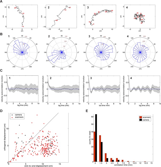
Figure 2. Trajectories of wild-type animals off food.

(A) Trajectories of representative wild-type animals on the camera set-up. Red dots on the trajectory indicate the position of the animal at 10-minute intervals. (B) Histograms of ‘radial displacements’ for the trajectories shown in (A). Counts within a bin are obtained by summing frame-to-frame displacements corresponding to instantaneous headings whose direction falls within the interval specified by the bin. Directions are relative to the set-up. (C) Heading autocorrelation function. The function is defined, for a lag time τ, as , where are the instantaneous unit direction vectors, and N is the total number of such vectors of the path. The function, smoothed with a cubic spline, is plotted in black; gray shading indicates the value of the signal +/- one standard deviation. (D) Scatter plot of the end-to-end displacement vs. the maximum displacement in the orthogonal direction for all trajectories. Red dots: scanner data. Black triangles: camera data. Black line: end-to-end displacement  =  orthogonal displacement. (E) Histogram of trajectory correlation times, defined as the first zero crossing of a path’s heading autocorrelation function. Red: scanner data-set; black: camera data-set. 75% of the scanner trajectories and 90% of the camera ones display correlation times of less than 3 minutes.