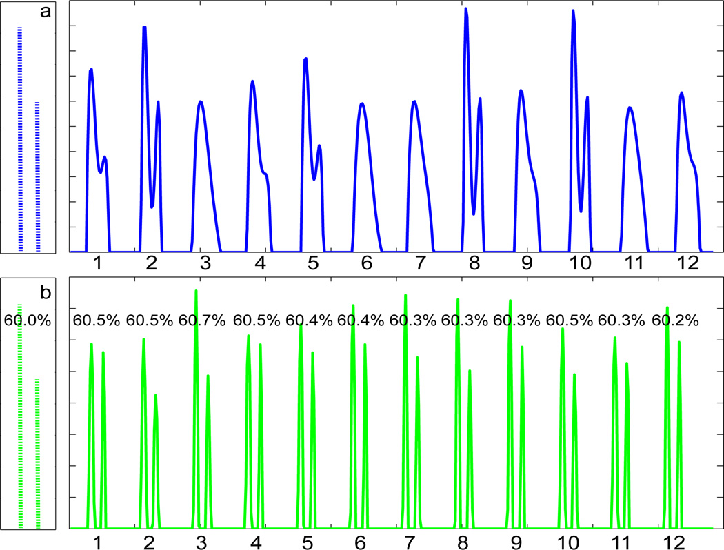
Figure 2.

The exact underlying form of a simulated distribution is shown on the left. The two components were defined by (T₂, weight) = (25 ms, 60%) and (35 ms, 40%). Relaxation data were generated from this and inverted using NNLS. Results from 12 different realizations of noise are shown on the right. a. Results from the 1D ILT (dashed arrow in Fig. 1). SNR = 15000. b. Results from 2DILTP (solid arrows in Fig. 1). T₁ values of 100 ms and 300 ms were assigned to the two components, respectively. $\mathrm{S}\mathrm{N}\mathrm{R}=15000\sqrt{6}~6000$. The numbers indicate the relative area of the larger component; all are within 1% of the correct value. Small variation in maxima is inherent to regularization.