Fig. 7.

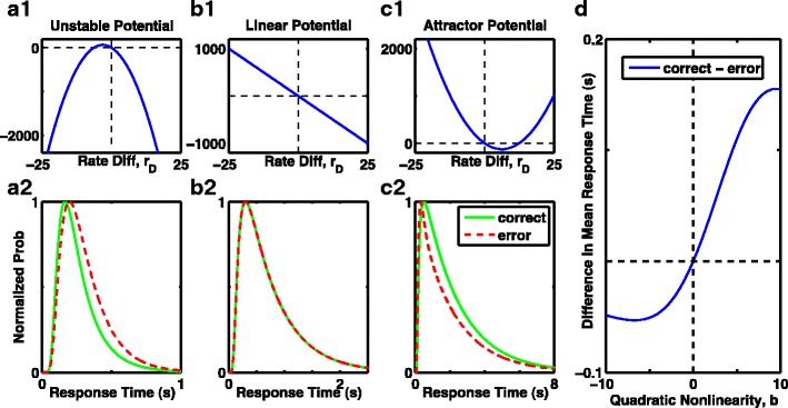
Expectation of faster or slower error responses depends on curvature of the nonlinear 1D model. a1), b1), c1) Effective potentials include a bias current, which produces correct responses at positive rate-difference r _D. a1) Fixed point of the unstable potential (where dr _D/dt = 0) is shifted left of the origin, so crossed on error but not correct trials, leading to slower error responses in a2. b1) Linear potential has constant gradient, leading to equal shapes of correct and error response distributions in b2. c1) Stable fixed point of the potential with a barrier is shifted to the right, so crossed on correct, but not error trials, leading to slower correct responses compared to errors in c2. a2), b2, c2) The corresponding response time distributions (scaled to a peak of 1, for easy comparison of the shapes—the number of errors is so much fewer than number of correct responses that shapes of the original distributions can not be visibly compared). Green solid curves: scaled distribution of correct response times. Red dashed curves: scaled distribution of error response times. a1), a2) b = −1. b1), b2) b = 0. c1), c2) b = 1. D Summary of the difference in mean response times as a function of quadratic curvature of the effective potential, or the stability of the initial fixed point (negative curvature is unstable, positive curvature is stable, zero curvature is marginally stable and equivalent to an integrator). Systems with an unstable fixed point produce slower errors, while systems with a stable fixed point produce faster errors. Simulations contained no fixed time limit, so a threshold was always reached