Figure 7.

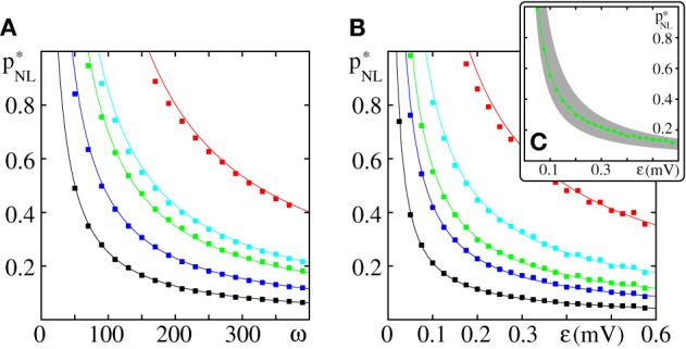
Critical connectivity in FFNs with non-linear dendrites. The panels show (A) the critical connectivity p^*_NL vs. the layer size ω for different coupling strengths (ϵ = {0.05 mV (red), 0.1 mV (cyan), 0.125 mV (green), 0.2 mV (blue), and 0.4 mV (black)}) and (B) p^*_NL vs. the coupling strength ϵ for different layer sizes (ω = {50 (red), 100 (cyan), 150 (green), 200 (blue), and 400 (black)}). The points indicate the minimal connectivity for which a synchronous pulse propagates from the first to the last layer in an FFN with m = 20 layers in at least 50% of n = 30 trials. The critical connectivity given by Equation (71) (solid lines) is in good agreement with the computer simulations. (C) The critical connectivity is confined to the interval p^*_NL ∈ [p⁰, 2p⁰] [indicated by the gray area for ω = 150 (green), cf. Equation (77)] and approaches its lower bound for small ϵ and its upper bound for large ϵ. Like in linearly coupled networks the critical connectivity decays inversely proportional to layer size, p^*_NL ∝ ω⁻¹, (cf. also Figure 3), but the scaling with coupling strength is more complicated, $p_{NL}^{\ast }\propto {ϵ}^{-1}·1/\beta \left(\frac{{\Theta }_b}{ϵ}\right)$; the factor $\beta \left(\frac{{\Theta }_b}{ϵ}\right)\in \left[0.5,1\right]$ [cf. Equation (70) and Figure 6] measures the deviation from the algebraic decay (as found in linearly coupled networks). In this figure the parameters of the external network are fixed to I₀ = 5 mV, ν^ext = 3 kHz, ϵ^ext = 0.5 mV.