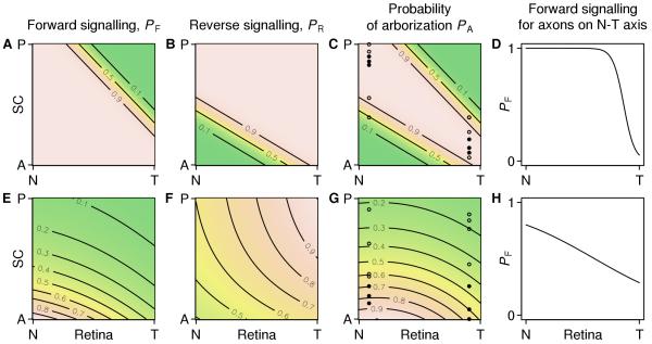
Figure 2. Arborization probabilities of axons from the retinal nasotemporal axis along the anterior-posterior axis of the SC.
A–D, The arborization probabilities plotted from equations in the Methods section of Grimbert & Cang (2012) and displayed in their Figure 2A–C. A, The forward arborization probability PF, which restricts arborizations from temporal axons in the posterior SC. B, the reverse arborization probability PR. C, the combined arborization probability PA, which is the product of PF and PR. Note that each axon is permitted to arborize in a region around its topographically appropriate location. The filled and open circles indicate the locations in the SC of arborizations from nasal and temporal axons generated by sampling from PA. There are seven points in total; in Grimbert & Cang’s simulations the arborizations with the four lowest values of PA (open circles) would be pruned leaving the three arborizations with the highest values of PA (filled circles). D, A nasotemporal slice of the forward arborization probability in A. E–H, Arborization probabilities computed by substituting plausible but unmatched gradients into the prescription in the Results section of Grimbert & Cang (2012). E, The forward arborization probability PF= 1/RF LF, where RF is the concentration of EphA receptor borne by an arbor and LF is the concentration of ephrin-A ligand it encounters at a location in the SC. Gradients are RF( x )= (1 .05+ 0. 26 exp( 2.3 x ))/1.05, where x= 0 is nasal and x= 1 is temporal (Reber et al., 2004), and LF( y )= exp(2. 1( y− 1)), where y= 0 is anterior and y= 1 is posterior. F, the reverse arborization probability PR and the concentrations RR and LR of ephrin-A and EphA are related similarly, with gradients RR( x )= 1+ 1.7 exp(− x) and LR( y )= 1+ 0.6 exp (− 2.6 y ) . G, the arborization probability computed from the product of PF and PR (E, F) and arborizations generated from the probability distribution as described in C. H, A nasotemporal slice of the plausible forward arborization probability, which is equal to 1/ RF( x) . Code to reproduce this figure is available in the Supplemental Information.

