Figure 7.

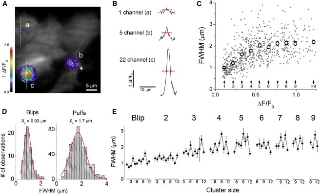
Dependence of spatial width (FWHM) of puffs on their amplitude. (A) Fluorescence image superimposing three puffs. Ca²⁺-fluorescence signals are depicted on a pseudocolor scale with “warmer” colors (grayscale in print) representing increasing ΔF/F₀. Images of the puffs were separately captured at the times of their peaks and are superimposed on a grayscale image of resting fluorescence to show cell outlines. Vertical lines indicate the locations of 3-pixel-wide regions used to generate fluorescence profiles as shown in B. (B) Examples of Ca²⁺-fluorescence profiles taken at the times of peak fluorescence of the events, estimated to involve 1 (a), 5 (b), and ∼22 (c) open channels. Event widths were measured at half-maximum amplitude, as indicated by the dashed horizontal lines. (C) Scatter plot showing the relationship between puff width (FWHM) and puff amplitude. Individual events are depicted as gray dots, plotted as a function of ΔF/F₀. Open circles show mean values pooled by the estimated number of channels open at the peak of the events. (D) Histograms showing the distributions of widths (FWHM) of blips (left, n = 80) and puffs (amplitudes ΔF/F₀ 0.165-2.54; right, n = 586). Curves are Gaussian fits. (E) Plots of mean event spatial widths (FWHM) as a function of cluster size, grouped by the estimated peak number of open channels during each event. To see this figure in color, go online.