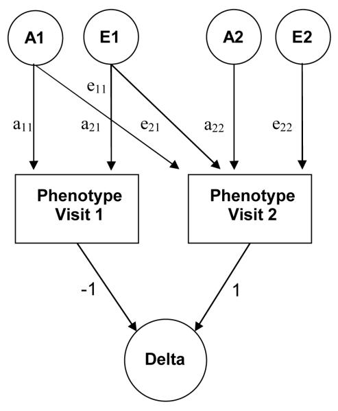
Figure 1.

Path diagram for a bivariate model.

For clarity only one twin is depicted. A1, A2 = Genetic variance components, E1, E2 = Non-shared environmental variance components, a₁₁ through a₂₂ = genetic path coefficients (or factor loadings) of which a₂₂ represents novel genetic influences on visit 2, e₁₁ through e₂₂ = non-shared environmental path coefficients. (or factor loadings) of which e₂₂ represents novel environmental influences on visit 2. Delta = difference in levels of measured phenotype between visit 2 and 1. Subtracting the level of the measured phenotype at time 2 from the level of the measured phenotype at time 1 is established by setting the path coefficients originating from the two measured phenotypes (and pointing towards delta) to -1 (time 1) and 1 (time 2).

Formulas for the different heritability estimates (listed in Table 5) are as follows:

• h² total (visit1) = a₁₁² / (a₁₁² + e₁₁²)
• h² total (visit2) = (a₂₁² + a₂₂²) / (a₂₁² + a₂₂² + e₂₁² + e₂₂²)
• h² specific (visit2) = a₂₂² / (a₂₁² + a₂₂² + e₂₁² + e₂₂²)
• h² delta (visit2 – visit1) = ((a₂₁- a₁₁)²+ a₂₂²) / ((a₂₁ - a₁₁)²+ a₂₂² + (e₂₁- e₁₁)²+ e₂₂²)