High-Resolution Free-Energy Landscape Analysis of α-Helical Protein Folding: HP35 and Its Double Mutant

Abstract

The free-energy landscape can provide a quantitative description of folding dynamics, if determined as a function of an optimally chosen reaction coordinate. Here, we construct the optimal coordinate and the associated free-energy profile for all-helical proteins HP35 and its norleucine (Nle/Nle) double mutant, based on realistic equilibrium folding simulations [Piana et al. Proc. Natl. Acad. Sci. U.S.A.2012, 109, 17845]. From the obtained profiles, we directly determine such basic properties of folding dynamics as the configurations of the minima and transition states (TS), the formation of secondary structure and hydrophobic core during the folding process, the value of the pre-exponential factor and its relation to the transition path times, the relation between the autocorrelation times in TS and minima. We also present an investigation of the accuracy of the pre-exponential factor estimation based on the transition-path times. Four different estimations of the pre-exponential factor for both proteins give k₀^–1 values of approximately a few tens of nanoseconds. Our analysis gives detailed information about folding of the proteins and can serve as a rigorous common language for extensive comparison between experiment and simulation.

1. Introduction

One of the reasons that the protein folding problem still interests researchers is that it is difficult to get direct and unambiguous answers about the basic questions of how proteins fold: What are the residual structure in denatured state, the nature of the folding steps, the free-energy landscape and kinetic barriers, transition path time, and pre-exponential factor? Widely differing opinions exist even for the fundamental issues and interpretation of many folding experiments.¹

Because of the limited spatial and temporal resolution of state-of-the-art experimental techniques, it is hard to obtain a direct detailed experimental characterization of the folding process. Many ingenious experimental approaches have been developed to overcome the shortcomings. Consider, for example, the problem of determining the folding free-energy barrier and the pre-exponential factor. While the folding rate can be measured directly, these quantities cannot. One approach considers “barrier-less” proteins, where the folding barrier is absent, and the pre-exponential factor closely approximates the folding time.^2,3 Another approach uses the relationship between the transition path times ⟨τ_TP⟩ and the pre-exponential factor derived for proteins with a simple landscape described by a single parabolic barrier between the native and denatured states.⁴ The highly nontrivial task of measuring directly the transition path times has been solved recently by direct counting of photons in single-molecule experiment.⁴ In another approach, a related quantity “molecular time” has been measured as a deviation from single exponential relaxation dynamics in a bulk temperature jump experiment.⁵ However, it is not clear how to directly verify experimentally that the protein landscape agrees with the assumed model form. In another attempt, the free-energy landscape of the PrP protein was reconstructed using force spectroscopy.⁶ However, direct interpretation of the results is complicated, because of the smoothing effect of the DNA handles and beads on dynamics, the perturbation of the landscape by the applied force, and the fact that the experimentally accessible reaction coordinate is not necessarily a “good” reaction coordinate. As a result, the obtained estimates for the pre-exponential factor and the transition path times have very large error margins. By measuring the contact formation times in unfolded polypeptides, a lower bound of k₀^–1 ≈ 10 ns has been suggested.⁷

In principle, the detailed picture of how proteins fold and, in particular, the estimation of the pre-exponential factor and transition-path times or the shape of the free-energy landscape, can be obtained by simulation. An additional advantage of such an approach is that it becomes possible to test the assumptions underlying the models used for the analysis of experimental data. However, until recently, such simulations faced three main challenges: the simulation time gap, accuracy of force fields and rigorous quantitative analysis of the obtained data.⁸⁻¹⁰ Recent advances in the computer hardware, simulation methodology, and force-field accuracy have made realistic simulation of the folding of small fast-folding proteins computationally affordable.¹¹⁻¹³ In particular, Lindorff-Larsen et al. reported the results of “brute-force” atomic-level MD simulations, of 12 fast-folding proteins.¹⁴

With the steady progress in the simulation of protein folding, the rigorous quantitative analysis of the obtained data becomes all the more important.⁹ The popular approaches are the Markov state models (MSMs),¹⁵⁻¹⁹ conformation network analysis,²⁰⁻²² and the free-energy landscape framework.²³⁻²⁸ The latter allows one to directly determine the major properties of the folding dynamics, namely, the folding free-energy barriers and the pre-exponential factor, the structure of the transition states (TS) and intermediates, the diffusion coefficient, and the transition path times. Determination of many of these properties with the alternative techniques is not straightforward. The most challenging part in the approach is the construction of the optimal reaction coordinate. A poorly chosen coordinate can hide the complexity of the dynamics,^8,25 decrease the height of the folding barrier, and make the dynamics subdiffusive.^27,29 In result, it may happen that analyses of the same trajectories, using the same framework, but with different methods produce different results.^13,27 The latter illustrates the importance of extensive, repetitive analysis of simulations.

Here, we apply a recently developed approach for the construction of the optimal reaction coordinate^27,30,31 to analyze the folding dynamics of the all-helical C-terminal fragment of villin headpiece (HP35) and its double norleucine mutant (Nle/Nle).³² The two proteins have been extensively studied by experiments³³⁻³⁸ and theory/simulations.^{8,14,32,39−46} In particular, an intermediate in wild-type HP35 was detected experimentally by solid-state NMR,³⁷ a triplet–triplet energy transfer (TTET) experiment,³⁶ and a simulation of an Ising type model of the protein.³⁵ Most of the experiments and simulations conclude that secondary structure and topology develop earlier than the full set of native contacts.^37,45 There is some disagreement on secondary structure formation; in particular, some results indicate that helices 1 and 2 are folded and helix 3 is unfolded in the intermediate state,^35,36 while MD simulations suggest an intermediate with helices 2 and 3 forming native interactions and helix 1 undocked.^40,41 Introduction of the stabilizing Nle-residues in helix 3 (the Nle/Nle mutant) increases the stability^33,34 and the folding rate, compared to those of the wild-type protein.^32,34 A rough estimate of k₀^–1 for HP35 double mutant of 420 ns was reported by Kubelka et al.³⁴

In this paper, we determine the optimal reaction coordinate and the associated free-energy profiles (FEP) for both proteins, which give a rigorous quantitative description of their folding dynamics. In particular, the secondary structure and hydrophobic core formations during the folding process are investigated and compared with experiment. The (folding) pre-exponential factor k₀ is estimated in four different ways. The estimates have the same order of magnitude (k₀^–1 ≈ 20 ns). In addition, we check the assumption used in the experimental estimate of k₀^–1, namely, that the correlation times at the TS and in the native state are the same.³⁴ The Appendix investigates the accuracy of the estimation of the pre-exponential factor from the transition-path times^4,32 for model systems. We believe that the detailed, rigorous analysis that has been presented allowed us to clarify the matter with the pre-exponential factor estimation.

2. Methods

The determination of the optimal reaction coordinate, which accurately represents the multidimensional folding dynamics, is the most challenging part of the approach. Once the coordinate has been determined, all the properties, such as the free-energy profile, the diffusion coefficient, and the structures are computed in straightforward manner with no further assumptions.

The putative reaction coordinate is taken as the (smoothed) number of contacts,²⁷

1

where r_ij is the distance between atoms i and j, defined as

h(x) is the (smoothed) Heaviside function (h(x) = min(1, max(x,0)), Δ_k is the threshold for the contact considered to be formed, and α_k is either +1 or −1. Two thousand (2000) contacts between H and O atoms are considered. Note that multiple contacts with the same atoms i_k and j_k but different Δ_k and α_k are possible, which makes the putative coordinate more flexible. Given the multidimensional simulation trajectory X(t) and putative reaction coordinate y (y = R(X)), one can compute the putative coordinate time series y(t) = R(X(t)), partition functions of conventional free-energy profile Z_H(y) and cut free-energy profiles Z_C(y) and Z_C,1(y).^30,31 The coordinate is optimized by numerically optimizing the parameters Δ_k, α_k, and (i_k, j_k), so that the functional ∫_A^Bdy/Z_C,1(y) computed for the trajectory is minimal, where A and B are positions of the minima in the native and denatured states. The optimization is performed with a penalty term to avoid overfitting. The detailed description of the stochastic optimization procedure, the penalty term, and the analysis of the robustness of the approach are reported in refs (27 and 30). Here, the robustness of the results was tested by repeating the optimization procedure, starting from different reaction coordinates (e.g., the root-mean-square deviation (rmsd) from the native state, the first principal component), using different seed numbers, all of which leading to the same results.

For an infinitely flexible reaction coordinate, the functional attains a minimum when the coordinate is equal to the (possibly rescaled) pfold coordinate R(X) = p_fold(X).³⁰ The dynamics projected on such a coordinate is diffusive and, together with the corresponding FEP and the diffusion coefficient, provides a complete and accurate description of the folding process.^27,31 In particular, the equilibrium folding flux can be computed exactly as diffusion on the free energy landscape.³¹ For a coordinate with finite approximation power, as considered here, the putative optimal coordinate approximates p_fold well only near the TS regions. However, these are the most important regions for folding kinetics, and such a coordinate is sufficient, for example, to directly determine the folding barrier and the pre-exponential factor.

Two thousand parameters were chosen, based on previous experience with analysis of a similar size protein.^27,30 While this number may seem very large, the following consideration shows that it is, in fact, quite modest. The reaction coordinate projects a trajectory with the length of a few million frames from a configuration space with dimension 3N – 6 (here 1725) onto a single coordinate. The optimal coordinate means that every configuration from the trajectory obtains the correct position after projection. Moreover, instead of using a specifically designed functional form with many parameters to better approximate the reaction coordinate, a linear combination of simple basis functions is used. Usage of the cut-profiles, which are invariant with respect to arbitrary rescaling of reaction coordinate, simplifies the problem since now every configuration should be in a correct order with respect to other configurations, rather than to have the correct absolute position.

That probably explains why such approach constructs the coordinates that are optimal only around the TS. In order to do this, one needs to solve two much simpler problems. First, remove all the points that belong to the minima from the TS region toward the corresponding minima; their precise position in the minima is not important. Second, correctly project the points that do belong to the TS region. Their number is usually orders of magnitude smaller than the trajectory length.

The position-dependent diffusion coefficient (D(y)) is directly determined as^30,31

After optimization, the putative optimal coordinate is rescaled by numerically integrating the expression

so that the diffusion coefficient is constant and equal to unity (D(z) = 1). In this case, the conventional profile

and the cut profile

differ by an unimportant constant. However, the cut profiles are less prone to statistical noise and are shown in the figures presented later in this work.

3. Results and Discussion

Simulation Detailes

Two simulation trajectories are analyzed: that of 398 μs for wild-type HP35 at T = 345 K and that of 301 μs for the (Nle/Nle) mutant at T = 380 K reported by Piana et al.³² The analysis is performed with a time resolution of Δt = 0.2 ns.

HP35 Wild-Type Villin: The Free-Energy Landscape

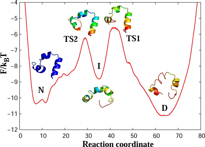
Figure 1 shows the FEP of wild-type villin HP35 as a function of the determined reaction coordinate. The landscape consists of five states: denatured basin (D), first transition state (TS1), intermediate state (I), second transition state (TS2), and native basin (N). The main folding barrier is the one between the denatured and intermediate states, with the height of ΔF/k_BT ≈ 5.5.

Figure 1.

Free-energy profile for wild-type villin (HP35) along the putative optimal reaction coordinate. [Legend: D, the denatured basin; I, the intermediate basin; N, the native basin; TS1, the first transition state; and TS2 the second transition state.] The main folding barrier between D and I states is ΔF/k_BT ≈ 5.5. The representative structures for the regions of the landscape show a trajectory snapshot closest to the average structure of the region. Colors code the root-mean-square (rms) fluctuations of atomic positions around the average structure from 1.5 Å (blue) to 7 Å (red).

At the denatured state, the protein is unstructured and generally lacks a helical secondary structure. The yellow color in the beginning of the third helix suggests that this part is more stable than the rest of the protein, while the red color shows large fluctuations of other parts of the protein. At TS1, helices 1 and 2 start to form (the green color indicates that fluctuations in these regions are decreasing). Full formation and stabilization of the second helix occurs at the intermediate state (green changes to blue). At TS2, the end of the C-terminal helix still fluctuates strongly (red color); however, all three helices are predominantly formed, showing the native-like structure of the protein, which is fully stabilized in the native state (deep blue color). Figure 2 shows representative conformers for each transition state.

Figure 2.

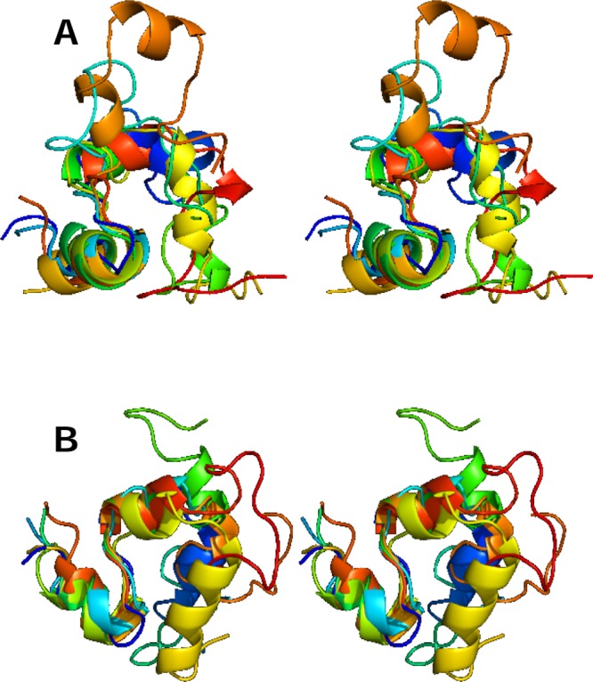
Stereo view of representative conformers for (A) TS1 and (B) TS2 transition states. Six conformers (for visual clarity) were randomly selected from each ensemble.

Secondary Structure Formation

Figure 3 shows the helical propensity (the fraction of time a residue is in a helical state) for different regions on the FEP and gives a detailed view on formation of helices during the folding process. In the denatured state (red line), the first and second helices are mainly unstructured (helical propensity of 20%–40%), while the beginning of the third helix (residues 63–66) is predominantly formed (60%). The red line shows that conformations with the joint first and second helices, as well as with the joint second and third helices, are possible.

Figure 3.

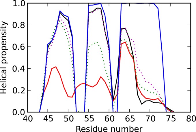
Helical propensity for different regions on the FEP. [Legend: the D state is shown by the red line, TS1 by the green dotted line, I state by the black line, TS2 by the magenta dotted line, and N state by the blue line.] The three helices in the native state are formed by residues 43–52, 54–59, and 62–73.

At TS1 (green dotted line) two separated helices form: part of helix 1 (residues 45–51) shows a helical propensity of 50%–80% and helix 2 shows 60%. Changes in the third helix are insignificant. The intermediate state (denoted by the black line) is characterized by stabilization of helix 2 with the helical structure observed in more than 90% of the snapshots. Surprisingly, the helical propensity of the end of helix 3 (residues 67–73) is lower, compared to that of the D state, and TS1 and shows nonmonotonic behavior. A similar analysis of the order of helix formation in wild-type villin shows that helix 2 forms first in 80% of the folding events.³² A triplet–triplet energy transfer (TTET) experiment³⁶ and a simulation of an Ising-type model of the protein³⁵ also indicate the presence of the intermediate state with helices 1 and 2 folded and helix 3 unfolded. These findings are in agreement with the presented results but in contrast to results from MD simulations that suggested an intermediate with helices 2 and 3 forming native interactions and helix 1 undocked.^40,41 At TS2 (denoted by the magenta dotted line), the turn between helix 2 and helix 3 forms and the third helix shows increased helical propensity at the end (residues 67–73). The latter is fully formed in the native state (blue line).

Hydrophobic Core Formation

A solid-state NMR experiment detected an intermediate state during HP35 folding with nearly native secondary structure but disordered tertiary structure.³⁷ In particular, starting with a thermally unfolded ensemble, a hydrophobic core formation of the HP35 folding process was investigated in unfolded, intermediate, and folded states. This experiment was carried out in a glycerol/water solution (the simulations were done in explicit water).

Figure 4A explores the formation of the hydrophobic core (residues Phe47, Val50, Phe51, Phe58, and Leu69) during the folding process. The snapshots show that the formation of native topology and secondary structure begins early during the folding process, while the stabilization of the hydrophobic core residues happens later. At the denatured state, unfolded protein has some helical content and a fully disordered tertiary structure. The intermediate state is characterized by the first and second helices formed but an incomplete hydrophobic core. The red and yellow colors of side-chains Val50 and Leu69 indicate large fluctuations of these residues. In the native state, the tightly packed hydrophobic core is fully formed. This finding reproduces the experimental results³⁷ and is in agreement with MD simulations, concluding that secondary structure and topology develop earlier than the full set of native contacts.³² Interestingly, the intermediate state contains conformations with a nearly native secondary structure and native-like topology (Figure 4B) but with an incompletely folded hydrophobic core.

Figure 4.

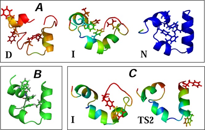
(A) Hydrophobic core formation during HP35 folding (the D state has a fully disordered tertiary structure; in the I state, the first and second helices formed but it still has an incomplete hydrophobic core; the N state has a tightly packed hydrophobic core). (B) A native-like structure with an incompletely folded hydrophobic core from the intermediate state (single snapshot). (C) Contact formation between side-chains Trp64 and Phe76 (the I state has contact between Trp64 and Phe76; the TS2 state shows the absence of Trp-Phe contact). The average configurations are taken from Figure 1.

Trp64 and Phe76 Contact Formation

The presence of an intermediate at the native side of the major folding/unfolding barrier in HP35 was suggested by an experiment using TTET to monitor conformational fluctuations.³⁶ In the intermediate state, the partially unfolded third helix is flexible enough to allow contact between side-chains Trp64 and Phe76, which is very unlikely in the native state. The experiment detected the presence of conformations without contact (I) and with contact (I*) in the intermediate state.

Our analysis confirms that the intermediate state contains both types of conformations. The distance between the residues fluctuates between 3.5 Å and 30 Å. The population of the conformations where Trp64 and Phe76 are in contact (Figure 4C) is approximately the same as the population of the conformations where these side-chains are apart (ratio 1:1.5). In contrast, TS2 is characterized by the absence of contact between Trp64 and Phe76 in most of the structures, with an average distance of 17–20 Å between these residues (Figure 4C). Structures with the interacting Trp and Phe are also present at TS2 but in a much smaller proportion (ratio is ∼1:15).

The schematic free-energy profile for the folding of wild-type HP35 at T = 300 K, with identified native (N) and near-native (N′) states, suggested in ref (36), differs from ours (Figure 1). One can attempt to extrapolate the profile to higher temperature. At the melting temperature, one would expect that the denatured and N′ states are equally populated while the N and I states are much less stable. It is also likely that the barrier between the denatured and intermediate states can become the rate limiting one. In this case, the profile will be similar to the one shown on Figure 1 if one assumes that N′ corresponds to N.

Nle/Nle Double Mutant

The HP35 protein contains two buried lysine residues at positions 65 and 70.

The high-resolution X-ray structure previously showed that removing the charge of Lys65 by substituting norleucine increases burial of the aliphatic side-chain of residue 65.³³ The stability of the mutant increases by 0.5 kcal/mol and additional mutation in residue 70 stabilizes the protein by another 0.5 kcal/mol.³⁴ Introduction of the stabilizing Nle-residues in helix 3 shifts the folding pathway relative to that in the wild-type protein.⁴³ In particular, it was found that helix 3 generally forms early during the folding path and helix 1 forms last.⁴⁵

The Free-Energy Landscape

Figure 5 shows the FEP of the Nle/Nle mutant as a function of the determined reaction coordinate. The FEP has one transition state (TS) between the denatured (D) and native (N) basins. The folding barrier of ΔF/k_BT ≈ 4.6 is lower than that of the wild type, reflecting the fact that the double mutant folds faster.^32,34

Figure 5.

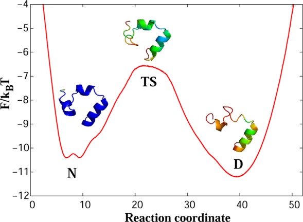
(A) Free-energy profile for the Nle/Nle mutant along the optimal reaction coordinate. D and N denote the denatured and native basins, respectively, while TS denotes the transition state.

Helix 3 is almost completely formed in the denatured state. The green color in the middle part of the helix indicates that this part is quite stable. The rest of the protein is unstructured (red and yellow colors suggest large fluctuations in the first and second helices). In the transition state, helix 2 forms (green color) and the protein takes near-native conformation (predominantly green and blue colors). In the native state, the protein is fully folded and stabilized (deep blue color). Figure 6 shows representative conformers of the TS ensemble.

Figure 6.

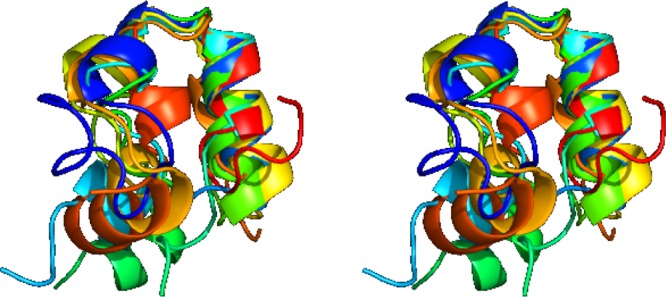
Stereo view of randomly chosen conformers from the TS ensemble of the Nle/Nle mutant.

An MSM analysis of a simulation of the Nle/Nle mutant with a ff9sb-ildn force field (the currently analyzed simulation used ff99sb*-ildn) and lower temperature (T = 360 K)⁴⁶ identified native N and near-native N′ states separated by a barrier. The latter, while being native-like, is characterized by partial unraveling of helix 3. The structural interpretation of both states was suggested to be close to those found in the TTET experiment of the wild-type HP35 at temperatures lower than 300 K.³⁶ However, our analysis suggests that the mutant has a simple landscape with just native and denatured basins and one transition state (Figure 5). Another coordinate optimized for the analysis of just the native basin found a small barrier of ΔF/k_BT ≈ 1.5. The conformations in two sub-basins differ mainly only by the orientation of side-chain Leu42 in the helix 1. The difference between our results and that of the MSM analysis can be due to different temperatures and force fields or due to the fact that while the major folding barrier can be easily identified, assignment and comparison of multiple small barriers is not so straightforward.

Secondary Structure Formation

Figure 7 shows how the helical propensity changes during folding. In the absence of an intermediate state, the plot shows monotonic behavior. In the denatured state (denoted by the red line), helix 3 is predominantly formed (helical propensity of 80%) with residues 67–73 having higher helical propensity (40%–60%), compared to the wild type. However, the structures with the joint second and third helices are still present in this state (helical propensity 10% in residues 61–62). Helices 1 and 2 are mainly unstructured. In the transition state (denoted by the green dotted line), the turn between the first two helices is well-defined and the propensity of both formed helices increases to 70%. The helical structure of helix 3 is present in 90% of the snapshots. Finally, all three helices are fully formed in the native state (denoted by the blue line).

Figure 7.

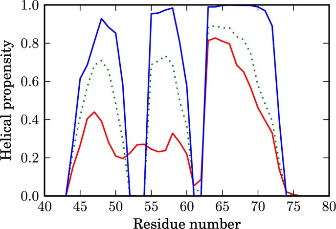
Helical propensity of the residues for different regions on the FEP. The D state is shown by the red line, the TS by the green dotted line, and the N state by the blue line.

Hydrophobic Core Formation

Figure 8 explores the hydrophobic core formation. The denatured state has helix 3 formed while the hydrophobic core residues are disordered. The red color shows strong fluctuations of the residues. In the transition state, the mutant exhibits a structure with native-like topology, the second and third helices are formed, and the hydrophobic core has almost packed. However, the red and yellow colors still indicate the presence of large fluctuations in Phe47 and Val50 side-chains. In the native state, tight packing of the phenylalanine residues completes the formation of the hydrophobic core.

Figure 8.

Hydrophobic core formation during the Nle/Nle double mutant folding.

Estimation of the Pre-exponential Factor k₀

We first report estimates of the pre-exponential factor (k₀) for the Nle/Nle mutant. It has a single TS, and the analysis is straightforward. The pre-exponential factor is estimated using four different approaches, with all results being in good agreement.

Estimate 1

The mean folding time or the mean first passage time (mfpt) from the denatured to the native state of the mutant estimated from the FEP by using Kramer’s equation is 1.6 μs. This value is lower than the folding time of τ_f = 3.0 μs, estimated directly from the trajectory. Such reasonable, although not ideal, agreement indicates that the FEP describes the kinetics reasonably well up to a factor of 2.

Using the height of the free-energy barrier between the D and N states (ΔF/k_BT = 4.6; recall Figure 5), the pre-exponential factor can be estimated from

2

as k₀^–1 ≈ 30 ns.

Estimate 2

Kramer’s equation for mfpt with harmonic approximation is^2,27

3

where ω_TS and ω_D are the curvatures of the TS and the D state, respectively, D_TS is the diffusion coefficient in the transition state, and β = 1/k_BT. The equation can be rearranged as²

4

Assuming ω_TS = ω_D, one obtains k₀^–1 = 2πτ_corr,TS, where τ_corr,TS = k_BT/(D_TSω_TS²) is the autocorrelation decay time at the transition state.^2,47,48 Note that the reaction coordinate is rescaled so that the diffusion coefficient D(x) = 1 (see Methods). The top of the transition state (Figure 5) is approximated by (ω_TS²/2)/k_BT ≈ 0.034, which leads to k₀^–1 ≈ 18 ns.

Estimate 3

Equation 3 can be rearranged in another way:²⁷

5

where Z_D is the total partition function of the denatured state, Z_C,TS is the cut profile at the top of the transition state (Z_C,TS = exp(F_C,TS/k_BT)), and Δt is the sampling interval. While this estimate also assumes that the profile at the TS is parabolic, it does not need the value of the curvature at the TS (as does the previous estimate): only the value of the cut profile Z_C,TS is needed. For the transition state (Z_C,TS = exp(6.6), Z_D = 1.1 × 10⁶) with Δt = 0.2 ns, one obtains τ_corr,TS ≈ 10.0 ns and k₀^–1 ≈ 63 ns.

In estimates 1–3, we used τ_f = 3.0 μs, obtained directly from the trajectory. Note, however, that if one uses the value estimated from the profile for the mfpt (i.e., 1.6 μs), then estimates 1, 2, and 3 give values of 16, 18, and 18 ns, respectively. Such a (superficially) good agreement is not surprising, since it is for a diffusive dynamics on the obtained FES, i.e., it just shows that the equations that have been derived are correct.

Estimate 4

A transition path is the part of the trajectory that crosses the reaction coordinate x at x₁ and reaches x₂ on the other side of the barrier without recrossing x₁.⁴⁹ The duration of this part is the transition-path time. The mean transition path times ⟨t_TP⟩, computed directly from the trajectory, can be used to estimate the pre-exponential factor using the relation⁵⁰

6

where k_f = 1/τ_f is the folding rate and γ ≈ 0.577 is Euler’s constant. The relation was derived assuming diffusive dynamics over a parabolic transition state with the height of the barrier being ΔF > 2k_BT.

We consider two cases: first, where boundaries x₁ and x₂ are placed on the FEP around the TS barrier, such that ΔF (ΔF = F_TS – F_xi) is 3k_BT and second, where x₁ and x₂ are taken at the minima of the denatured and native basins, correspondingly. The measured ⟨t_TP⟩ values are 14.6 and 62.4 ns, respectively, with the corresponding k₀^–1 values (eq 6) being 33.3 and 169.5 ns. The first number agrees with the other estimates, while the second is much larger. An analysis of the model systems (see the Appendix) shows that the estimate of k₀ with eq 6 is the most accurate when transition path times are calculated between x₁ and x₂ with ΔF ≈ 3k_BT; that, in our case, corresponds to k₀^–1 ≈ 33.3 ns.

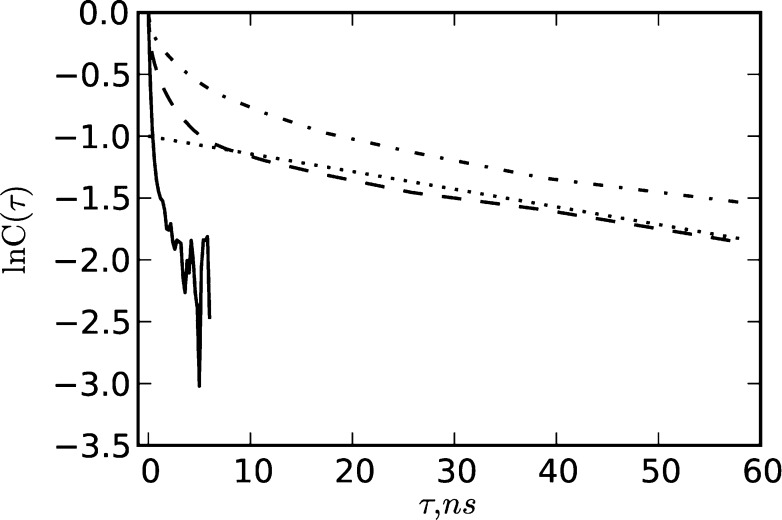
Experimental estimates of k₀ for the Nle/Nle double mutant were obtained by Kubelka et al.³⁴ A “very rough estimate” was made by assuming that the empirical protein folding “speed limit” t_f = N/100 μs, where N is the number of residues in the polypeptide chain,² corresponds to k₀^–1; for N = 35, one obtains k₀^–1 ≈ 350 ns. The second estimate is based on the decay time of the autocorrelation function in the folded state. A value of τ_corr = 70 ns was obtained from a biexponential fit of the relaxation after a temperature jump.³⁴ Assuming that the decay times in the native and transition states are the same (i.e., that these states have similar curvature and diffusion coefficients), one finds k₀^–1 = 2πτ_corr ≈ 420 ns. Having the folding trajectory, we can test the assumptions: in particular, how similar are the autocorrelation decay times at different regions on the FEP? Figure 9 shows the logarithm of the position autocorrelation function ln C(τ) in the N, D, and TS states, where

and

As one can see, the autocorrelation function does not have a simple single-exponential decay C(τ) = exp(−τ/τ_corr), and, thus, τ_corr cannot be unambiguously determined. However, it is clear that the “effective” decay time at the transition state, which actually determines the pre-exponential factor, is significantly smaller than that in the basins, indicating that the assumption above is likely to be poor. Note that the long-time slope of lnC(τ) in the D and N states is close to the experimentally measured τ_corr value (τ_corr = 70 ns).

Figure 9.

Plot of the position autocorrelation function in the native (N) state (dashed line), the denatured (D) state (dash-dotted line), and the transition state (TS) (solid line). Dotted line shows ln C(τ) = −1 – τ/70, which is an autocorrelation function with a time decay τ_corr = 70 ns to mimic the experiment.³⁴

Estimation of k₀ for HP35

The wild-type protein has two free-energy barriers, where one is lower than the other. The pre-exponential factor of only the main folding barrier between D and I states is considered. The mfpt value needed to overcome the first folding barrier, computed directly from the trajectory, is τ = 9.2 μs. The mfpt value estimated from the FEP is τ = 3.75 μs, which indicates that the FEP describes the dynamics relatively well. Using eq 2 with ΔF/k_BT = 5.5, one finds k₀^–1 ≈ 35 ns.

The curvature of the first transition state (ω_TS²/2)/k_BT ≈ 0.056 gives k₀^–1 ≈ 11 ns. Using eq 5 with Z_D = 1.41 × 10⁶ and Z_C,TS = exp(5.6), one obtains τ_corr,TS ≈ 7.8 ns and k₀^–1 ≈ 49 ns.

For estimate 4, we, analogously, consider several cases where x₁ and x₂ are placed at 3k_BT from the top of the first transition barrier, at the minima of the D and I states and at the minima of the D and N states, correspondingly. The ⟨t_TP⟩ values are 12.8, 200, and 753 ns with corresponding k₀^–1 = 26.3, 555, and 2380 ns. Piana et al. determined the mean transition path times between the folded and unfolded states to be 120 ns < ⟨t_TP⟩ < 460 ns, which gives pre-exponential factor estimates of 500 ns < k₀^–1 < 1500 ns.³² These upper and lower boundaries are close to our estimates of k_0,DI^–1 ≈ 555 ns and k_0,DN^–1 ≈ 2380 ns. However, the analysis of such estimation for model systems presented in the Appendix shows that the transition path times are very sensitive to the exact nature of the landscape and the positions of the boundaries. In particular, it is shown that the most accurate estimate of the pre-exponential factor is obtained when x₁ and x₂ are taken around the main transition state at positions with energy of ∼3k_BT, which is less than that of the barrier. In our case, it corresponds to k₀^–1 ≈ 26 ns. If the region between the boundaries contains multiple, even relatively small barriers, the transition path times are dominated by the waiting time in the “intermediate” states. They no longer measure just the time required to cross the barrier and, hence, are no longer directly related to k₀.

Reiner et al.³⁶ estimated the rates of loop formation between all three helices in the denatured state for wild-type HP35 at T = 25 °C to be ∼10⁷ s^–1. Assuming that the rate of loop formation is higher at higher T = 380 K and that the pre-exponential factor is somewhat faster than the rate of the complete loop formation, one can expect an estimate close to the one obtained here. A related estimate for the pre-exponential factor k₀^–1 ≈ 10 ns obtained from the rates of contact formation in short polypeptides⁷ is in agreement with ours.

4. Conclusion

The free-energy profiles for all-helical proteins, HP35 and its Nle/Nle double mutant, along the putative optimal reaction coordinate have been determined. The coordinates, together with the associated FEPs and diffusion coefficient, provide an accurate description of the folding dynamics of these proteins and allow direct estimation of the transition path times and the pre-exponential factor. The analysis shows that HP35 folds through an intermediate. In particular, the intermediate is characterized by the second and first helices formed but with an incomplete hydrophobic core that quantitatively reproduces the NMR experiment.³⁷ The second transition state describes the folding of helix 3. It has been also observed that, because of the fluctuations of helix 3, the intermediate state contains structures with and without contact between side-chains Trp64 and Phe76, in agreement with the TTET experiment.³⁶ The Nle/Nle mutant with two stabilizing residues in helix 3 has a simple landscape with only one transition state. Helix 3 is mostly folded in the denatured state and it appears that single TS (where helices 1 and 2 cooperatively fold) is sufficient to complete the folding process. A lower free-energy barrier also leads to faster folding dynamics in agreement with previous studies. The pre-exponential factor k₀ was estimated in four different ways all giving the same order of k₀^–1 ≈ 20–50 ns.

In summary, significant recent advances in computational power, accuracy of the force field and simulation methodology have made possible the realistic simulation of relatively fast-folding proteins. Rigorous free-energy landscape analysis of such simulations gives a detailed quantitative picture of how proteins fold and allows direct determination of many of the basic properties of protein folding dynamics, some of which can be estimated experimentally, only in an indirect way.

Appendix

Estimations of the Pre-exponential Factor Using the Transition Path Times

Two model systems are considered to investigate the accuracy of the estimations of the pre-exponential factor.

Consider a 1D model system with potential energy profile U₁(x) = 2.5 cos[(4xπ/50) – 2π] for x ∈ [0,50] (see Figure A1). The trajectory was generated by simulating Metropolis Monte Carlo (MC) dynamics with Gaussian steps corresponding to D(x) = 1 for 1.5 × 10⁶ steps. The time step is considered to be 1 ns for straightforward comparison with the MD simulations. Figure A1 shows the free-energy profile along the reaction coordinate (rescaled such that D(x) = 1) determined from the generated trajectory. The FEP is very similar to the model potential U₁(x). The small difference is due to a slight underestimation of the diffusion coefficient, which leads to expansion of the reaction coordinate during rescaling.

Figure A1.

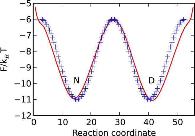
Model potential U₁(x) = 2.5 cos[(4xπ/50) – 2π] (blue crosses) and the free-energy profile along the reaction coordinate determined from the trajectory, generated by simulating MC on the potential (red line). The model potential U₁(x) is shifted along the axes.

The pre-exponential factor k₀^–1 estimated from the barrier height ΔF/k_BT = 5 and the mfpt of 7.6 μs (eq 2) is 51 ns. The curvature of the transition state is approximated by (ω_TS²/2)/k_BT = 0.066, which leads to k₀^–1 ≈ 48 ns (eq 4). The value of ω_TS²/2 computed analytically for U₁(x) is 0.078, which gives the estimation of k₀^–1 ≈ 40 ns. The value of k₀^–1 computed from eq 5 is 47 ns (Z_D = 7.95 × 10⁵, Z_C,TS = exp(6.0) ≈ 403).

The transition path times, computed for several choices of boundaries x₁ and x₂ are shown in Table A1. With the distance from the transition state increasing (larger ΔF/k_BT), the transition path time increases from 26.2 ns to 53.6 ns and the corresponding pre-exponential factor increases from 57.8 ns to 125.8 ns. Comparing these values with the k₀^–1 value calculated using other estimations above, one can see that the closest estimate is obtained when ΔF = 3k_BT. However, all values are of the same order of magnitude. Thus, for the FEP with the single parabolic barrier, the estimates of ⟨t_TP⟩ and corresponding k₀^–1 are not very sensitive to the exact position of the boundaries, or to the height of the barrier.⁴ In this case, the values of the pre-exponential factor estimated by eq 6 differ just by a factor of 2. The advantage of such an estimate is that one does not need to know the exact barrier height to determine the optimal reaction coordinate. However, a landscape of the model system is too simple.

Table A1. Dependence of Transition Path Times ⟨t_TP⟩ and Corresponding k₀^–1 on the Positions of the Boundaries x₁ and x₂ on the FEP.

x1	x2	⟨tTP⟩ (ns)	k0–1a (ns)	ΔF/kBTb
36	19.8	26.2	57.8	3
37.8	17.8	32.2	72	4
41.6	14.2	53.6	125.8	5

^ak₀^–1 is the pre-exponential factor estimated from eq 6.

^bΔF/k_BT is the height of the barrier from the position x₁ or x₂ to the transition state.

Model system 2 has an additional barrier in the “native” state with the following potential energy profile for x ∈ [0,50] (Figure A2):

The trajectory was generated analogous to the above for 1.5 × 10⁶ steps. Figure A2 shows the free-energy profile constructed using the generated trajectory.

Figure A2.

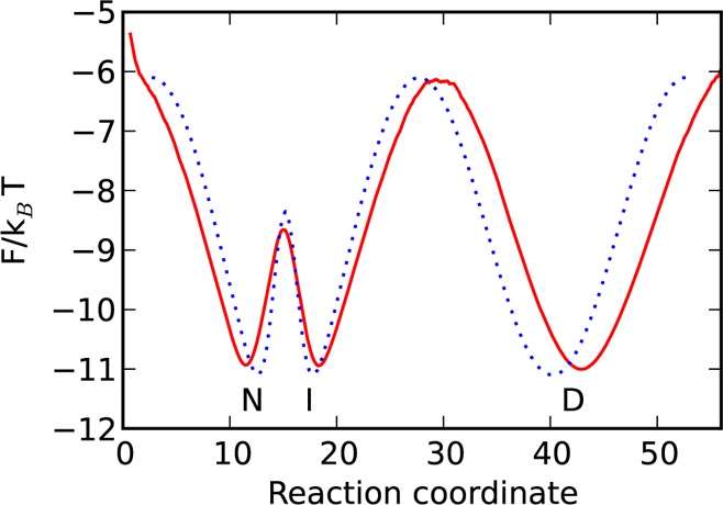
Model potential with two barriers U₂(x) (denoted by the blue dotted line) and the free-energy profile along the reaction coordinate determined from the trajectory (denoted by the red line).

The second barrier is much smaller than the first barrier and, hence, does not change the folding–unfolding times significantly: 7.36 μs, calculated from the D state to the I state vs 7.7 μs calculated from the D state to the N state. The pre-exponential factor k₀^–1 estimated from eq 2 is 57 ns (the height ΔF/k_BT = 4.9 and mfpt τ = 7.7 μs). The top of the transition state is approximated by ((ω_TS²/2)/k_BT) = 0.063, which leads to k₀^–1 ≈ 50 ns calculated from eq 4. k₀^–1 computed from eq 5 is 66 ns (Z_D = 7.5 × 10⁵, Z_C,TS = exp(6.1) ≈ 446)). The three estimates are in good agreement.

The transition path times, computed for several choices of boundaries x₁ and x₂, are shown in Table A2. When the segment between x₁ and x₂ includes just one barrier, the estimate is close to the correct value. Inclusion of the second barrier leads to much larger values of ⟨t_TP⟩ ≈ 125.7–160 ns and k₀^–1 ≈ 322–435 ns, correspondingly. The latter is due to the fact that, in the case of two barriers, the transition path times are dominated by the waiting time in the “intermediate” state. They no longer measure just the time required to cross the barrier and, hence, are no longer directly related to k₀. Thus, for complex landscapes, the estimated value of 6 can significantly overestimate k₀, if multiple barriers (even relatively small) are present in the segment. Knowledge of the optimal reaction coordinate and the associated FEP can be used to place the boundaries x₁ and x₂ just around the main barrier and, thus, improve the accuracy of the estimate.

Table A2. Dependence of Transition Path Times ⟨t_TP⟩ and Corresponding k₀^–1 on the Position of Boundaries x₁ and x₂ on the FEP.

x1	x2	⟨tTP⟩ (ns)	k0–1a (ns)	ΔF/kBTb
37.6	21.8	24.5	53.5	3
39.7	20.3	31.4	70	4
42.8	18.5	43.4	100	5
37.6	14.2	125.7	322.5	3
39.7	13.0	147.8	394	4
42.8	11.6	160	435	5

^ak₀^–1 is the pre-exponential factor estimated from eq 6.

^bΔF/k_BT is the height of the barrier from the position x₁ or x₂ to the transition state.

The authors declare no competing financial interest.

References

- Sosnick T. R.; Barrick D. The folding of single domain proteins – have we reached a consensus?. Curr. Opin. Struct. Biol. 2011, 21, 12–24. [DOI] [PMC free article] [PubMed] [Google Scholar]
- Kubelka J.; Hofrichter J.; Eaton W. A. The protein folding “speed limit”. Curr. Opin. Struct. Biol. 2004, 14, 76–88. [DOI] [PubMed] [Google Scholar]
- Yang W. Y.; Gruebele M. Folding at the speed limit. Nature. 2003, 423, 193–197. [DOI] [PubMed] [Google Scholar]
- Chung H. S.; McHale K.; Louis J. M.; Eaton W. A. Single-molecule fluorescence experiments determine protein folding transition path times. Science. 2012, 335, 981–984. [DOI] [PMC free article] [PubMed] [Google Scholar]
- Liu F.; Nakaema M.; Gruebele M. The transition state transit time of WW domain folding is controlled by energy landscape roughness. J. Chem. Phys. 2009, 131, 195101-1–195101-7. [DOI] [PubMed] [Google Scholar]
- Yu H.; Gupta A. N.; Liu X.; Neupane K.; Brigley A. M.; Sosova I.; Woodside M. T. Energy landscape analysis of native folding of the prion protein yields the diffusion constant, transition path time, and rates. Proc. Natl. Acad. Sci. U.S.A. 2012, 109, 14452–14457. [DOI] [PMC free article] [PubMed] [Google Scholar]
- Krieger F.; Fierz B.; Bieri O.; Drewello M.; Kiefhaber T. Dynamics of unfolded polypeptide chains as model for the earliest steps in protein folding. J. Mol. Biol. 2003, 332, 265–274. [DOI] [PubMed] [Google Scholar]
- Freddolino P. L.; Harrison C. B.; Liu Y.; Schulten K. Challenges in protein folding simulations: Timescale, representation, and analysis. Nat. Phys. 2010, 6, 751–758. [DOI] [PMC free article] [PubMed] [Google Scholar]
- Lane T. J.; Shukla D.; Beauchamp K. A.; Pande V. S. To milliseconds and beyond: Challenges in the simulation of protein folding. Curr. Opin. Struct. Biol. 2013, 23, 58–65. [DOI] [PMC free article] [PubMed] [Google Scholar]
- Best R. B. Atomistic molecular simulations of protein folding. Curr. Opin. Struct. Biol. 2012, 22, 52–61. [DOI] [PubMed] [Google Scholar]
- Freddolino P. L.; Liu F.; Gruebele M.; Schulten K. Ten-microsecond molecular dynamics simulation of a fast-folding WW domain. Biophys. J. 2008, 94, L75–L77. [DOI] [PMC free article] [PubMed] [Google Scholar]
- Ensign D. L.; Pande V. S. The fip35 WW domain folds with structural and mechanistic heterogeneity in molecular dynamics simulations. Biophys. J. 2009, 96, L53–L55. [DOI] [PMC free article] [PubMed] [Google Scholar]
- Shaw D. E.; Maragakis P.; Lindorff-Larsen K.; Piana S.; Dror R. O.; Eastwood M. P.; Bank J. A.; Xumper J. M.; Salmon J. K.; Shan Y.; Wriggers W. Atomic-level characterization of the structural dynamics of proteins. Science 2010, 330, 341–346. [DOI] [PubMed] [Google Scholar]
- Lindorff-Larsen K.; Piana S.; Dror R. O.; Shaw D. E. How fast-folding proteins fold. Science 2011, 334, 517–520. [DOI] [PubMed] [Google Scholar]
- Noé F.; Fischer S. Transition networks for modeling the kinetics of conformational change in macromolecules. Curr. Opin. Struct. Biol. 2008, 18, 154–162. [DOI] [PubMed] [Google Scholar]
- Bowman G. R.; Beauchamp K. A.; Boxer G.; Pande V. S. Progress and challenges in the automated construction of markov state models for full protein systems. J. Chem. Phys. 2009, 131, 124101-1–124101-11. [DOI] [PMC free article] [PubMed] [Google Scholar]
- Pande V.; Beauchamp K.; Bowman G. Everything you wanted to know about Markov state models but were afraid to ask. Methods 2010, 52, 99–105. [DOI] [PMC free article] [PubMed] [Google Scholar]
- Prinz J.-H.; Wu H.; Sarich M.; Keller B.; Senne M.; Held M.; Chodera J. D.; Schütte C.; Noé F. Markov models of molecular kinetics: Generation and validation. J. Chem. Phys. 2011, 134, 174105-1–174105-23. [DOI] [PubMed] [Google Scholar]
- Prinz J.-H.; Keller B.; Noé F. Probing molecular kinetics with Markov models: Metastable states, transition pathways and spectroscopic observables. Phys. Chem. Chem. Phys. 2011, 13, 16912–16927. [DOI] [PubMed] [Google Scholar]
- Rao F.; Caflisch A. The protein folding network. J. Mol. Biol. 2004, 342, 299–306. [DOI] [PubMed] [Google Scholar]
- Prada-Gracia D.; Gómez-Gardeñes J.; Echenique P.; Falo F. Exploring the free energy landscape: From dynamics to networks and back. PLoS Comput. Biol. 2009, 5, e1000415. [DOI] [PMC free article] [PubMed] [Google Scholar]
- Dickson A.; Brooks C. L. Native states of fast-folding proteins are kinetic traps. J. Am. Chem. Soc. 2013, 135, 4729–4734. [DOI] [PMC free article] [PubMed] [Google Scholar]
- Onuchic J. N.; Socci N. D.; Luthey-Schulten Z.; Wolynes P. G. Protein folding funnels: The nature of the transition state ensemble. Folding Des. 1996, 1, 441–450. [DOI] [PubMed] [Google Scholar]
- Dobson C. M.; Sali A.; Karplus M. Protein folding: A perspective from theory and experiment. Angew. Chem., Int. Ed. 1998, 37, 868–893. [DOI] [PubMed] [Google Scholar]
- Krivov S. V.; Karplus M. Hidden complexity of free energy surfaces for peptide (protein) folding. Proc. Natl. Acad. Sci. U.S.A. 2004, 101, 14766–14770. [DOI] [PMC free article] [PubMed] [Google Scholar]
- Best R. B.; Hummer G. Reaction coordinates and rates from transition paths. Proc. Natl. Acad. Sci. U.S.A. 2005, 102, 6732–6737. [DOI] [PMC free article] [PubMed] [Google Scholar]
- Krivov S. V. The free energy landscape analysis of protein (FIP35) folding dynamics. J. Phys. Chem. B 2011, 115, 12315–12324. [DOI] [PubMed] [Google Scholar]
- Rohrdanz M. A.; Zheng W.; Maggioni M.; Clementi C. Determination of reaction coordinates via locally scaled diffusion map. J. Chem. Phys. 2011, 134, 124116-1–124116-11. [DOI] [PubMed] [Google Scholar]
- Krivov S. V. Is protein folding sub-diffusive?. PLoS Comput. Biol. 2010, 6, e1000921. [DOI] [PMC free article] [PubMed] [Google Scholar]
- Krivov S. V. Numerical construction of the pfold (committor) reaction coordinate for a Markov process. J. Phys. Chem. B. 2011, 115, 11382–11388. [DOI] [PubMed] [Google Scholar]
- Krivov S. V. On reaction coordinate optimality. J. Chem. Theory Comput. 2013, 9, 135–146. [DOI] [PubMed] [Google Scholar]
- Piana S.; Lindorff-Larsen K.; Shaw D. E. Protein folding kinetics and thermodynamics from atomistic simulation. Proc. Natl. Acad. Sci. U.S.A. 2012, 109, 17845–17850. [DOI] [PMC free article] [PubMed] [Google Scholar]
- Chiu T. K.; Kubelka J.; Herbst-Irmer R.; Eaton W. A.; Hofrichter J.; Davies D. R. High-resolution X-ray crystal structures of the villin headpiece subdomain, an ultrafast folding protein. Proc. Natl. Acad. Sci. U.S.A. 2005, 102, 7517–7522. [DOI] [PMC free article] [PubMed] [Google Scholar]
- Kubelka J.; Chiu T. K.; Davies D. R.; Eaton W. A.; Hofrichter J. Sub-microsecond protein folding. J. Mol. Biol. 2006, 359, 546–553. [DOI] [PubMed] [Google Scholar]
- Kubelka J.; Henry E. R.; Cellmer T.; Hofrichter J.; Eaton W. A. Chemical, physical, and theoretical kinetics of an ultrafast folding protein. Proc. Natl. Acad. Sci. U.S.A. 2008, 105, 18655–18662. [DOI] [PMC free article] [PubMed] [Google Scholar]
- Reiner A.; Henklein P.; Kiefhaber T. An unlocking/relocking barrier in conformational fluctuations of villin headpiece subdomain. Proc. Natl. Acad. Sci. U.S.A. 2010, 107, 4955–4960. [DOI] [PMC free article] [PubMed] [Google Scholar]
- Hu K.-N.; Yau W.-M.; Tycko R. Detection of a transient intermediate in a rapid protein folding process by solid state nuclear magnetic resonance. J. Am. Chem. Soc. 2010, 132, 24–25. [DOI] [PMC free article] [PubMed] [Google Scholar]
- Serrano A. L.; Bilsel O.; Gai F. Native state conformational heterogeneity of HP35 revealed by time-resolved FRET. J. Phys. Chem. B 2012, 116, 10631–10638. [DOI] [PMC free article] [PubMed] [Google Scholar]
- Ensign D. L.; Kasson P. M.; Pande V. S. Heterogeneity even at the speed limit of folding: Large-scale molecular dynamics study of a fast-folding variant of the villin headpiece. J. Mol. Biol. 2007, 374, 806–816. [DOI] [PMC free article] [PubMed] [Google Scholar]
- Lei H.; Wu C.; Liu H.; Duan Y. Folding free-energy landscape of villin headpiece subdomain from molecular dynamics simulations. Proc. Natl. Acad. Sci. U.S.A. 2007, 104, 4925–4930. [DOI] [PMC free article] [PubMed] [Google Scholar]
- Yang J. S.; Wallin S.; Shakhnovich E. I. Universality and diversity of folding mechanics for three-helix bundle proteins. Proc. Natl. Acad. Sci. U.S.A. 2008, 105, 895–900. [DOI] [PMC free article] [PubMed] [Google Scholar]
- Lei H.; Deng X.; Wang Z.; Duan Y. The fast-folding HP35 double mutant has a substantially reduced primary folding free energy barrier. J. Chem. Phys. 2008, 129, 155104-1–155104-7. [DOI] [PMC free article] [PubMed] [Google Scholar]
- Lei H.; Chen C.; Xiao Y.; Duan Y. The protein folding network indicates that the ultrafast folding mutant of villin headpiece subdomain has a deeper folding funnel. J. Chem. Phys. 2011, 134, 205104-1–205104-7. [DOI] [PMC free article] [PubMed] [Google Scholar]
- Beauchamp K. A.; Ensign D. L.; Das R.; Pande V. S. Quantitative comparison of villin headpiece subdomain simulations and triplet-triplet energy transfer experiments. Proc. Natl. Acad. Sci. U.S.A. 2011, 108, 12734–12739. [DOI] [PMC free article] [PubMed] [Google Scholar]
- Piana S.; Lindorff-Larsen K.; Shaw D. E. How robust are protein folding simulations with respect to force field parameterization?. Biophys. J. 2011, 100, L47–L49. [DOI] [PMC free article] [PubMed] [Google Scholar]
- Beauchamp K. A.; McGibbon R.; Lin Y.-S.; Pande V. S. Simple few-state models reveal hidden complexity in protein folding. Proc. Natl. Acad. Sci. U.S.A. 2012, 109, 17807–17813. [DOI] [PMC free article] [PubMed] [Google Scholar]
- Buchner G. S.; Murphy R. D.; Buchete N.-V.; Kubelka J. Dynamics of protein folding: probing the kinetic network of folding-unfolding transitions with experiment and theory. Biochim. Biophys. Acta 2011, 1814, 1001–1020. [DOI] [PubMed] [Google Scholar]
- Best R. B.; Hummer G. Coordinate-dependent diffusion in protein folding. Proc. Natl. Acad. Sci. U.S.A. 2010, 107, 1088–1093. [DOI] [PMC free article] [PubMed] [Google Scholar]
- Hummer G. From transition paths to transition states and rate coefficients. J. Chem. Phys. 2004, 120, 516–523. [DOI] [PubMed] [Google Scholar]
- Chung H. S.; Louis J. M.; Eaton W. A. Experimental determination of upper bound for transition path times in protein folding from single-molecule photon-by-photon trajectories. Proc. Natl. Acad. Sci. U.S.A. 2009, 106, 11837–11844. [DOI] [PMC free article] [PubMed] [Google Scholar]