Fig. 2.

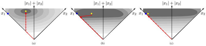
Geometry of convex objective functions for BP, CBP-T, and CBP-P methods, illustrated in two dimensions. Signal consists of a single waveform, f(t − 0.65Δ), and the dictionary contains two shifted copies of the waveform, {f(t), f(t − Δ)}, along with interpolating functions appropriate for each method. Each plot shows the space of coefficients, {x₁, x₂}, associated with the two shifted waveforms. Contours of gray-scale regions indicate level surfaces of reconstruction error (L₂ norm term of the objective function). The blue star indicates the true L₀-minimizing solution. The L₁ sparsity measure is the sum of the two coefficient values, corresponding to the vertical position on the plot. Red curve indicates family of solutions traced out as λ is increased from 0 (yellow dot) to infinity. Red points along this path indicate equal increments in reconstruction accuracy, with enlarged point indicating a common value for comparison across all three methods. (a) Standard BP solution (Eq. (7)). (b) Continuous basis pursuit with Taylor interpolator (Eq. (13)), using a basis of {f₀, $f_0^{\prime }$, f_Δ, $f_{\mathrm{\Delta }}^{\prime }$}. In this case, the iso-accuracy contours are computed by minimizing the L₂ error over all feasible values of the derivative coefficients, and are thus no longer elliptical. (c) CBP with polar interpolation (Eq. (20)).