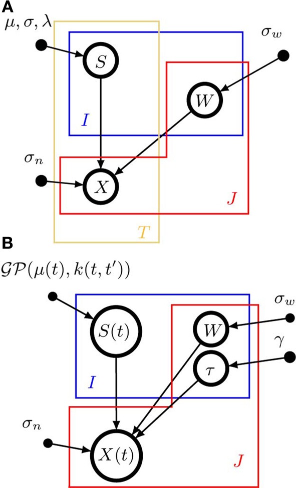
Figure 1.

Graphical model representations of the blind source separation algorithms for which we compute a model evidence approximation. We follow standard graphical modeling terminology (see e.g., Bishop, 2007). Open circles represent random variables, which may also be random functions. Filled circles are parameters. Arrows denote conditional dependencies. The plates (colored frames) indicate that the enclosed structure is repeated as often as the corresponding letter indicates. Enclosure in multiple plates indicates a product of repetitions. For example, in panel (A) there are I × T random variables S which comprise the source matrix. (A) Instantaneous, undelayed mixtures such as pPCA (where λ = 0) and ICA. J × T signals X are computed by mixing I × T sources S with J × I weights W. σ_w is the standard deviation of the zero-mean Gaussian prior on the weights. σ_n is the noise standard deviation. μ and σ are the parameters of the Gaussian part of the prior on the sources, λ measures the deviation from Gaussianity. (B). Convolutive, delayed mixtures, like the anechoic mixture of Omlor and Giese (2011) with additional temporal smoothness constraints. I source functions S(t) are drawn from a Gaussian process (μ(t), k(t, t′)) with mean function μ(t) and kernel k(t, t′). These sources are shifted in time by J × I many delays (one per trial and source) drawn from an exponential distribution with parameter γ and mixed with J × I weights W which are drawn from a zero-mean Gaussian distribution with standard deviation σ_w, to yield J signals X(t). For details, see text.