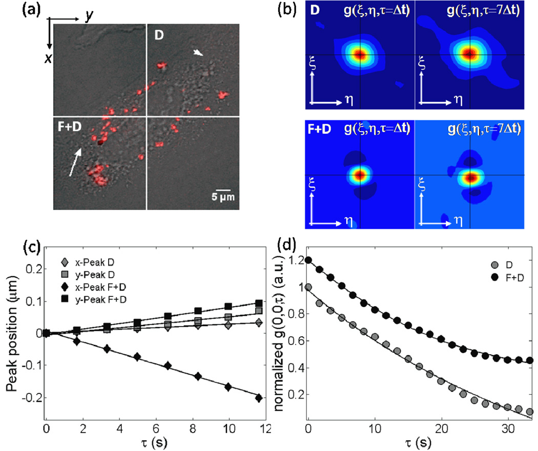
Figure 2.
Division of figure 1a into four ROIs as small as 128 × 128 pixels each (a). The steps of our analysis as proposed in figure 1, but restricted only to the top-right and bottom-left ROIs.(b) contour plots of the raw STICS curves at τ=Δt and τ=7Δt; the top and bottom plots refer to the top-right and bottom-left 128× 128 pixels ROIs of (a), respectively. (c) thex- and y-coordinates (filled diamonds and squares, respectively) of the 2D Gaussian peak position as a function of the delay time τ. Solid line is the best linear fit to the data. From the slope of the linear fits, the velocities (νSTICS) along the x- and y- directions could be calculated. From them, we can classify the top-right and bottom-left ROIs motion as diffusion (D) and flow and diffusion (F+D), respectively. The division in four smaller ROIs allows mapping of the lipoplex flow field; the velocity vectors are inserted in the corresponding ROI (white arrows). (d) fitting for the raw temporal image correlation functions (filled circles) using the proper theoretical model (equations (4) and (6) for D and F+D, respectively).

