Abstract
We present an approach for segmenting the left ventricular endocardial boundaries from radio-frequency (RF) ultrasound. The method employs a computationally efficient two-frame linear predictor which exploits the spatio-temporal coherence of the data. By performing segmentation using the RF data we are able to overcome problems due to image inhomogeneities that are often amplified in B-mode segmentation, as well as provide geometric constraints for RF phase-based speckle tracking. We illustrate the advantages of our approach by comparing it to manual tracings of B-mode data and automated B-mode boundary detection using standard (Chan and Vese-based) level sets on echocardiographic images from 28 3D sequences acquired from 6 canine studies, imaged both at baseline and 1 hour post infarction.
1 Introduction
Myocardial strain and strain rate measurements have been shown to be important for understanding cardiac disease. To this end, it has been reasonably well established that speckle tracking from high frame-rate radio-frequency (RF) ultrasound data can be used to generate dense estimates of displacement that can be used to solve for strain [1]. Current speckle tracking algorithms suffer from two drawbacks. First, they are extremely computationally intensive. Second, they perform well only on spatially homogeneous regions of the myocardium, but cannot easily identify such regions.
Segmentation of the left ventricle is particularly challenging in echocardiography due to gross inhomogeneities present in the images that lead to poor contrast between the blood and myocardium, as demonstrated in [2]. Analysis of high frame-rate (30 fps) raw RF images may provide important features that can be exploited to segment these regions. The primary benefit of using RF as opposed to B-mode images for boundary detection is that, due to the regular structure of the myocardium, the phase of the RF exhibits a temporal coherence not present in the blood pool. This phase information is exploited by looking at complex correlations in state-of-the-art speckle tracking, and its advantages over B-mode are documented in the ultrasound physics literature [1]. This suggests an advantage in using RF data for segmentation. Direct segmentation of the RF also provides a mask that indicates volumes where meaningful cardiac speckle tracking results can be expected and thus a means of simplifying computations.
Few segmentation methods thus far have leveraged RF data for boundary discrimination. Yan et al. [3] and Nillesen et al. [4] use maximum correlation coefficient (MCC) images obtained from RF speckle tracking to segment the left ventricle. These methods suffer from the fact that precomputation of the MCC images is extremely computationally burdensome. Alternatively, Dydenko et al. [5] propose both a spectral autoregressive model and a velocity based model for tissue discrimination. The authors of [5] also establish the variance of the velocity as a meaningful parameter for segmentation.
The key observation in all of the above research is that the temporal correlation in the blood pool and myocardium have different patterns. We also exploit this effect, although we use a model that is computationally much simpler than calculating the MCC image, i.e., linear prediction. Experimental observation shows that this simple model, as opposed to more complex motion models, provides accurate segmentations. This is the main contribution of this paper. We also propose the use of the residues of a linear predictor as a basis for segmentation. These residues are similar to the variance of the velocity adopted in [5]. In addition, as opposed to the single-frame autoregressive model [5], a two-frame linear predictor is more useful because, while the autoregressive fit will vary wildly across the image, the temporal coherence in the signal leads to a more consistent fit that can be used to segment the whole boundary. We adopt a maximum a posteriori (MAP) approach to the segmentation with a probabilistic model that relates subsequent frames of a cardiac image sequence. This estimation is performed numerically by means of a level set active contour. We compare our method to a traditional Chan-Vese intensity based level set segmenter on B-mode images [6]. Additional validation is performed by comparison with manual segmentations.
2 Materials and Methods
2.1 Signal Model
Data Set
The interaction of the base-band RF signal with two specific acoustic media (blood pool and myocardium) is of interest for this work. The blood pool is made up of plasma and other elements that are much smaller than the wavelength of the ultrasound, while the myocardium is made up of primarily muscular fibers interspersed with blood vessels and bile ducts. The fibers make up 90% of the myocardial tissue and are thus responsible for most of the received signal [7]. The regular structure of the fibers is responsible for the temporal coherence in the data that we exploit with our algorithm. Likewise, the lack of regular structure in the blood pool causes the signal to rapidly decorrelate.
It is of particular interest to us that our data is acquired at a high frame rate so that the motion of the speckle between frames is not significant relative to the boundaries. As a result, a single linear predictor for each medium (blood pool and myocardium) suffices for segmentation. Because of this, our algorithm is computationally efficient.
Preprocessing
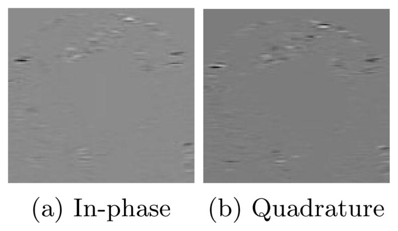
The input pulse produced by the ultrasound machine is a real, bandlimited signal. Since the effects of transmission and reflection in ultrasound are linear, the signal we record is also real and bandlimited and can thus be recovered by coherent demodulation [8]. The demodulation results in a vector image consisting of an in-phase and quadrature component and is referred to as the analytic signal. It is this vector image we are interested in segmenting. An example analytic image is shown in Figure 3.
Fig. 3.

Slice of analytic image containing myocardium and blood pool
2.2 Linear Predictor
Let IA be the 3D frame we wish to segment and IB be the subsequent 3D frame. The domain of IA is Ω and C is a boundary between two disjoint regions in the image, ΩC and Ω̃C, where Ω = ΩC ∪ Ω̃C. Then the absolute linear prediction residue of the mth voxel is
| (1) |
Note that voxels in ΩC and Ω̃C have different predictor coefficients; these are given by vectors α, β, α̃, and β̃ indexed by n where defines the nth neighbor of voxel , and . A diagram of the predictor is shown in figure 1.
Fig. 1.

Linear Predictor for point m
2.3 MAP Estimation
We assume that em for m ∈ ΩC and m′ ∈ Ω̃C are distributed normally with probabilities p1and p2, zero mean, and standard deviations σ1and σ2, respectively. We seek to segment the image within a level set formulation. Let φm : Ω →
 be the level set function whose zero level set is C, and let H be a smooth Heaviside function. Segmentation is performed by maximizing the following log posterior probability with α, β, α̃, and β̃ as defined in equation 1:
| (2) |
2.4 Level Set Formulation of the Model
Maximizing the likelihood is equivalent to minimizing its negative, so we define our energy functional as E(em, φm, α, α̃, β, β̃, σ1, σ2) = −l(em, φm, α, α̃, β, β̃, σ1, σ2). As in [6], we introduce a standard prior on the arc length of the propagating front, Eprior (φm). Finally, we introduce a prior on the smoothness of the predictor parameters given by ES (α, α̃, β, β̃) = α⊤Wα + α̃⊤Wα̃+ β⊤Wβ+ β̃⊤Wβ̃ where W is a finite difference matrix. The overall energy is thus given by E(em, φm, α, α̃, β, β̃, σ1, σ2) = ELP(em, φm, α, α̃, β, β̃, σ1, σ2) + λprior Eprior(φm) + +λSES(α, α̃, β, β̃) where λS and λprior are weights on the smoothness priors.
2.5 Optimization
We minimize the energy functional as follows: 1) Initialize φ inside the blood pool. 2) Update the other (non-level set) parameters of the model. 3) Update φ. We then iterate steps 2 and 3 until a local minima of the energy functional is reached. φ is updated by gradient descent, while the other parameters admit closed form solutions.
The maximum likelihood estimates of σ 1 and σ 2 are given by the standard formula for normally distributed random variables. Solving for the predictor parameters requires accumulating the voxels of IA to form the vectors xA and yA that contain the values of all of the real and imaginary ordered voxels in ΩC. x̃A and ỹA are likewise formed from voxels in Ω̃C. Similarly, the matrices XB, YB, X̃B, and ỸB are generated by defining the rows as the real and imaginary values of the neighborhoods of all ordered voxels in IB. The estimates for the prediction parameters are thus given by the following matrix equations, referred to as the normal equations:
| (3) |
| (4) |
| (5) |
| (6) |
These equations minimize the sum of squared differences between the in-phase and quadrature predictions.
3 Experiments
We acquired 28 sequences of canine RF images from 6 studies using a Phillips iE33 4D Ultrasound imaging system with a sampling rate of 30 frames per second. These images came from both healthy and diseased animals. 15 sequences were acquired at baseline while 13 sequences were acquired one hour post infarction. The infarction was performed by angioplasty occlusion. The proposed algorithm was evaluated at both end-diastole and a frame from ventricular ejection as these time points represent both the minimum and maximum average motion of the left ventricle, respectively. To preserve image acquisition statistics for this analysis and future speckle tracking, the images were left in the Frustum coordinate system, which consists of one scan line dimension and two angular dimensions.
To evaluate the algorithm and compare it with standard techniques, two algorithms were implemented: 1) The Chan-Vese algorithm [6]; 2) Our algorithm based on linear prediction. The Chan-Vese algorithm assumes intensity is homogeneous over each region of the image and only assumes a smoothness prior for the boundary. To properly leverage the temporal continuity in myocardial speckle, the search window for the coefficients of the predictor was chosen such that it included the maximum observed distance between any given speckle in two frames (typically on the order of 30 voxels in the axial dimension and 4 in each angular dimension). This window size is fixed for all experiments. Then, to further reduce complexity, the number of coefficients was decimated so each coefficient represented multiple voxels.
3.1 The Advantage of Segmenting Based on Temporal Coherence
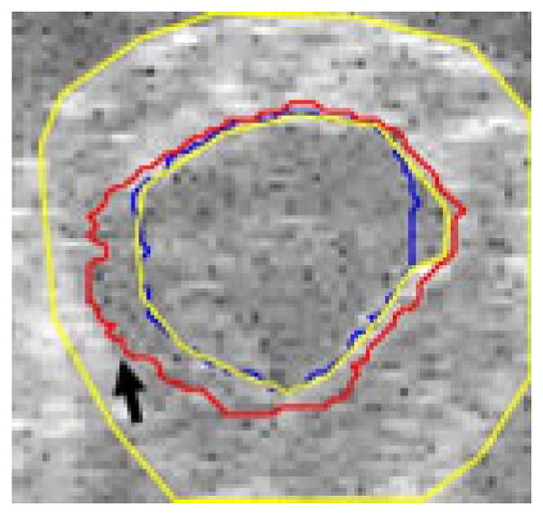
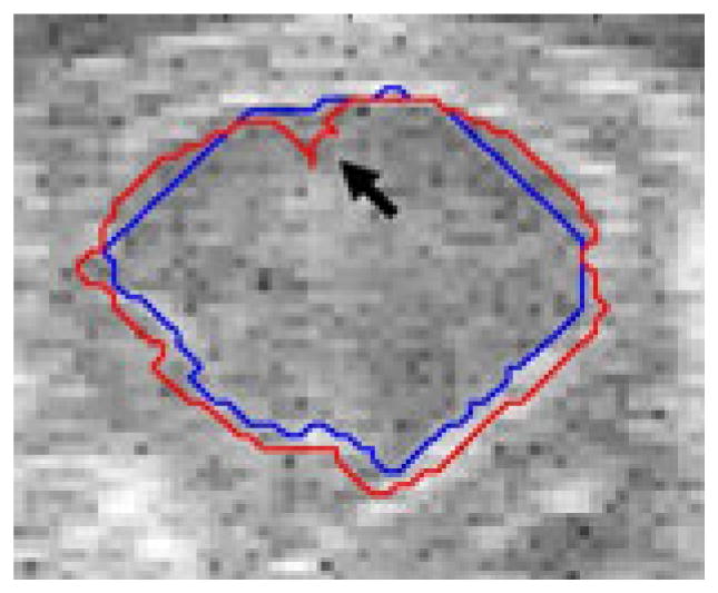
Examples of the performance of the algorithms are shown in figures 2, 4, and 5. The results for the Chan-Vese algorithm are shown in red and our results are shown in blue. In figure 2a, both contours underestimate the boundary on either side of the papillary muscle, but while the proposed algorithm underestimates this boundary to a more significant degree, the Chan-Vese contour leaks out through a mild dropout in the image that does not affect the results of our algorithm. Similar results are shown in figures 2b and 2c for images that contains more significant signal dropout.
Fig. 2.

Chan-Vese contours leak out
Fig. 4.

Chan-Vese contour fails to find boundary
Fig. 5.

Chan-Vese contour adheres to acquisition artifact
Figure 4 shows an example image where, due to poor contrast, the Chan-Vese algorithm fails to adhere to the endocardial border and instead adheres to the inside of the specularity produced by the epicardium, while our proposed algorithm finds the appropriate boundary (true boundaries in yellow). In the image in figure 5 there is an artifact present in the image that leads to a bright spot in the blood pool. Our proposed algorithm finds the correct boundary in the presence of this artifact, while the Chan-Vese contour adheres to the artifact.
3.2 Results
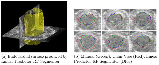
We compared our algorithm and the Chan-Vese algorithm with manually segmented surfaces. Typical segmentations are shown in figures 6a and 6b. Examples showing how the three contours compare are shown in figure 6b for visual evaluation. It was observed by visual inspection that, for most of our data sets, the Chan-Vese model overestimated the size of the blood pool. The error in the proposed model appears to be related to an underestimation of the extent of the blood pool in localized regions.
Fig. 6.

Typical segmentations
To quantitatively evaluate the results, we utilized the following three segmentation quality indices: 1) Huasdorff Distance (HD); 2) Mean Absolute Distance (MAD); and 3) the Dice coefficient. It should be noted that 8 Chan-Vese segmentations leaked, failing to find the endocardium, and were thus not included in the quantitative analysis.
Sequences obtained at baseline and those obtained one hour post infarct produced no significant difference in any of the quality indices, so all of the sequences were used to generate the values in Tables 1 and 2.
Table 1.
Sample means and standard deviations of quality indices (n=28) for segmentations obtained on frames at end diastole
| Chan-Vese | Proposed Algorithm | |||||
|---|---|---|---|---|---|---|
| Performance Measures | Dice | HD | MAD | Dice | HD | MAD |
| Average | 0.643 | 11.885 | 1.862 | 0.725 | 11.436 | 1.983 |
| STD | 0.048 | 4.526 | 0.377 | 0.061 | 1.943 | 0.349 |
Table 2.
Sample means and standard deviations of quality indices (n=28) for segmentations obtained on frames from ventricular ejection
| Chan-Vese | Proposed Algorithm | |||||
|---|---|---|---|---|---|---|
| Performance Measures | Dice | HD | MAD | Dice | HD | MAD |
| Average | 0.653 | 9.823 | 1.812 | 0.723 | 9.426 | 1.872 |
| STD | 0.036 | 4.732 | 0.497 | 0.056 | 2.936 | 0.363 |
HD and MAD did not differ greatly between the methods. This result can be explained by the fact that both methods often produce smooth curves that were close to the ground truth with the Chan-Vese contour overestimating and our method slightly underestimating the dimension of the blood pool. As such, the most useful measure in evaluating our method is the Dice coefficient where our algorithm showed a marked improvement over the Chan-Vese method.
Analysis of frames at end diastole and during ventricular ejection produced similar results which demonstrate our proposed algorithm functions both during minimum and maximum motion of the ventricle, which respectively correspond to maximum and minimum temporal coherence in the signal.
4 Discussion and Conclusions
We have presented an active contour RF ultrasound segmentation model that leverages temporal linear prediction within an image sequence. The algorithm relies solely on features present in the signal rather than a priori knowledge of expected shape. By utilizing a feature for segmentation that does not make a piecewise homogeneous assumption for the image, our contour is prevented from leaking out through boundaries that have relatively poor contrast. Since the motion of blood is irregular, performing speckle tracking on the blood pool provides no meaningful information. Our objective function segments based on the same concept, so it is particularly well suited for providing a geometric constraint for RF speckle tracking.
We also showed that our algorithm performs well during both peak and minimum average motion of the ventricle. Thus the algorithm can be extended to segment entire 4D data sets. Nonetheless, solving for the predictor coefficients is not trivial. An extension of this method to larger data sets, 4D segmentation, and joint endocardial/epicardial segmentation will require modifying this stage of the algorithm. This will be accomplished by gradient descent or the Levenberg-Marquardt algorithm.
Other future work includes validation of prediction coefficients and an analysis of their contribution, as opposed to residues, to segmentation. Also, the assumption of a fixed neighborhood for the linear predictor breaks down near the epicardial boundary causing a slight underestimation of the blood pool, which will be addressed through minor changes to our model. Ultimately, this method will be integrated as a preprocessing step into RF speckle tracking algorithms.
Acknowledgments
The authors would like to thank Matt O’Donnell, University of Washington, for helpful discussions and the reviewers for critical feedback.
Footnotes
This work is supported by grants 5R01HL082640-04 and 5R01HL077810-04.
References
- 1.Lubinski M, Emelianov S, O’Donnell M. Speckle tracking methods for ultrasonic elasticity imaging using short time correlation. IEEE trans Ultrason Ferroelect Freq Control. 1999;46:82–96. doi: 10.1109/58.741427. [DOI] [PubMed] [Google Scholar]
- 2.Qian X, Tagare HD. Overcoming dropout while segmenting cardiac ultrasound images. ISBI. 2006:105–108. [Google Scholar]
- 3.Yan P, Jia CX, Sinusas A, Thiele K, O’Donnell M, Duncan JS. LV Segmentation through the analysis of radio frequency ultrasonic images. Inf Process Med Imaging. 2007;20:233–244. doi: 10.1007/978-3-540-73273-0_20. [DOI] [PubMed] [Google Scholar]
- 4.Nillesen M, Lopata RGP, Huisman HJ, Thijssen JM, Kapusta L, Korte CL. 3D cardiac segmentation using temporal correlation of radio frequency ultrasound data. In: Yang G-Z, Hawkes D, Rueckert D, Noble A, Taylor C, editors. MICCAI 2009. LNCS. Vol. 5762. Springer; Heidelberg: 2009. pp. 927–934. [DOI] [PubMed] [Google Scholar]
- 5.Dydenko I, Friboulet D, Gorce JM, D’Hooge J, Bijnens B, Magnin IE. Towards ultrasound cardiac image segmentation based on the radiofrequency signal. Med Image Anal. 2003;7(3):353–367. doi: 10.1016/s1361-8415(03)00010-0. [DOI] [PubMed] [Google Scholar]
- 6.Chan TF, Vese LA. Active Contours Without Edges. IEEE Transactions on Image Processing. 2001;10:266–277. doi: 10.1109/83.902291. [DOI] [PubMed] [Google Scholar]
- 7.Shung K, Thieme G. Ultrasonic scattering in biological tissues. CRC Press; Boca Raton: 1993. [Google Scholar]
- 8.Langton C. Hilbert transform, analytic signal, and the complex envelope. Signal Processing and Simulation Newsletter. 1999 [Google Scholar]


