MODELING LONGITUDINAL MRI CHANGES IN POPULATIONS USING A LOCALIZED, INFORMATION-THEORETIC MEASURE OF CONTRAST

Abstract

Longitudinal MR imaging during early brain development provides important information about growth patterns and the development of neurological disorders. We propose a new framework for studying brain growth patterns within and across populations based on MRI contrast changes, measured at each time point of interest and at each voxel. Our method uses regression in the LogOdds space and an information-theoretic measure of distance between distributions to capture contrast in a manner that is robust to imaging parameters and without requiring intensity normalization. We apply our method to a clinical neuroimaging study on early brain development in autism, where we obtain a 4D spatiotemporal model of contrast changes in multimodal structural MRI.

1. INTRODUCTION

Longitudinal imaging during early brain development provides important information about normative patterns of growth, neuro-developmental disorders, and the link between brain and behavior. Early growth involves several rapid biophysical, chemical, structural, and functional changes which occur in an extremely organized and predictable manner. Myelination, or the formation of a myelin sheath around a nerve fiber, is a crucial part of the maturation processes as it facilitates the effective transmission of neural impulses [1]. It has been observed through qualitative findings that early growth and maturation, as a result of myelination, is marked by continuous changes in Magnetic Resonance Imaging (MRI) intensity [2].

In comparison to brain images from other modalities such as Computed Tomography (CT) and ultrasound, T1 Weighted (T1W) and T2 Weighted (T2W) MR images are ideal for assessment of growth as they exhibit much higher contrast sensitivity [2]. Higher signal intensities in T1W MR images, and lower signal intensities in T2W MR images, are shown to be the results of myelination. Rather than tracking appearance based changes, most existing studies of the pediatric brain have focused mainly on volumetric and morphometric indicators [3]. Recently, appearance based research restricted to signal intensity changes in MR images of the pediatric brain showed interesting results [4, 5]. However, the limitations of intensity based studies include excessive dependence on the use of accurate intensity normalization, and sensitivity to factors such as type of scanner and pulse sequence used in MR acquisition. Other existing studies on image contrast are based on ratios of image intensities which can be affected by population variabilities and imaging parameters [6].

Our recent method quantified contrast by using a distance metric between image histograms to measure the overlap between the intensity histograms of white and gray matter tissue classes in major brain regions [7]. This involved the challenging task of intensity normalization of the T1W and T2W MR images over a period marked by rapid contrast and appearance changes. In the current paper, we propose a new method for measuring contrast in longitudinal MRI that does not require intensity normalization procedures. In addition, changes are measured in populations at the full spatiotemporal level, where contrast is measured at every time point and for every voxel as opposed to specific regions. The new method uses tissue probability maps to measure local contrast via the Kullback-Leibler (KL) information theoretic measure. Thus, it does not rely on intensity normalization and it is more robust to changing imaging parameters (e.g., in multi-site imaging studies). We model population growth by conducting kernel regression on the tissue probability maps which results in continuous 4D models of change for every subject. We present results that demonstrate the application of our method for comparing different population groups as well as temporal changes within one population.

2. METHOD

We propose a new framework for studying brain growth patterns within and across populations based on contrast changes. We assume all multimodal longitudinal images have been registered to a common coordinate space. Probability maps for relevant tissue classes are computed at the time points scanned, which are then interpolated at time-points of interest using a continuous spatiotemporal modeling method. Contrast is measured at interpolated time points at every voxel as the information theoretic divergence measure between the mean distribution in the voxel neighborhood and the distributions at the neighboring voxels. Comparison statistics are then performed on these contrast measures.

2.1. Continuous 4D Spatio-Temporal Probability Maps

In this study, we make use of existing segmentations that are represented as sets of probability maps of major tissue classes. Our method can make use of any segmentation procedures and it is not restricted to specific segmentation approaches. Given a segmented image I of a subject s scanned at time t_i, we compute the subject-specific data likelihood for a tissue class c as p(I_s|c, μ_c, Σ_c) = (μ_c, Σ_c), where denotes a normal distribution with mean μ_c and covariance Σ_c. Therefore, the probability mass functions (pmf) P_s(c|x, t_i) can be estimated for every voxel x, subject s, and tissue class c from the likelihood values, as: $P_s(c\mid I_s(x,t_i),{\mu }_c,{\mathrm{\sum }}_c)=\frac{p(I_s\mid c,{\mu }_c,{\mathrm{\sum }}_c)}{{\sum }_{c^{\prime }}p(I_s\mid c^{\prime },{\mu }_{c^{\prime }},{\mathrm{\sum }}_{c^{\prime }})}$.

We perform kernel regression to obtain the probability mass functions at specific time points in a continuous manner. The regression is performed on the LogOdds transformed probabilities to take advantage of the linear/vector space operations in this space [8]. The pmf at a specific time point is then computed as the inverse map of the regression of LogOdds values that is guaranteed to be a proper distribution. In the case of multiple label classification, the LogOdds representation is defined as the ratio between the probability of a class c and the class c_BG representing background [9]:

$$L_s(c\mid x,t_i)=\mathit{log}\left(\frac{p(c\mid x,t_i)}{p(c_{BG}\mid x,t_i)}\right).$$ (1)

The interpolated LogOdds representation of the probabilities L_s(c|x, t) for a subject s are generated for time t as a continuous function through kernel regression on the individual probability values of each voxel in the LogOdds space:

$$L_s(c\mid x,t)=\frac{{\sum }_{t_i}K(t,t_i)L_s(c\mid x,t_i)}{{\sum }_{t_i}K(t,t_i)},$$ (2)

where K(t, t_i) is a smooth kernel. Finally, by taking the inverse of L_s using the inverse LogOdds function, we obtain values in the space of probability distributions:

$$P_s(c\mid x,t)=\{\begin{array}{cc}\frac{\mathit{exp}(L_s(c\mid x,t))}{Z}& c\ne c_{BG}\\ 1/Z& c=c_{BG}\end{array}$$ (3)

where Z = 1 + Σ_c≠cBG exp(L_s(c|x, t)).

2.2. Information Theoretic Contrast Measure

We generate a measure of contrast from the tissue class probability maps by calculating the mean of the distributions in a voxel neighborhood and the distance to the mean using the Kullback-Leibler (KL) divergence. The mean of the voxel neighborhood is computed to be the distribution which minimizes the sum of the weighted KL distance of all voxels in the neighborhood to itself. Given the probability map information in a voxel’s neighborhood, the KL divergence measures the deviation of the neighboring voxels from the typical distribution. Consider a voxel x in an image s such that the voxels in its neighborhood are denoted by y ∈ (x). The weight w_y of each voxel y is a function that varies inversely with its distance from x. The weighted mean of the probability mass functions of all voxels y in the neighborhood of x is known to be the weighted normalized geometric mean:

$${\overline{P}}_s(c\mid x,t)=\frac{1}{Q}{\left(\prod _{y\in \mathcal{N}(x)}{P}_s{(c\mid y,t)}^{w_y}\right)}^{\frac{1}{{\sum }_{y\in \mathcal{N}(x)}{w}_y}}$$ (4)

where Q denotes the sum of the geometric mean over all the classes. Contrast γ at a voxel x and time t is then measured as the weighted KL divergence:

$$\gamma (x,t)=\sum _{y\in \mathcal{N}(x)}w(y)KL\left({\overline{P}}_s(c\mid x,t),P_s(c\mid y,t)\right)$$ (5)

Regions with good contrast have bimodal probability distributions that represent mixed tissue, hence displaying higher KL divergence. Conversely, regions with low contrast have lower KL divergence as the distributions are unimodal and tight.

2.3. Analysis of Growth through Contrast

We conduct quantitative analysis of growth using these 4D values of contrast. Our method enables standard statistical approaches such as two sample t-test to determine significant differences between two population groups at a specific time point. Another approach is to measure changes between different time points within a single group to isolate significant variations across time. These statistical comparisons are conducted with correction for multiple comparisons using the False Discovery Rate (FDR) method [10].

3. RESULTS

Our method is applied to clinical longitudinal data obtained from the ACE-IBIS (Autism Centers of Excellence, Infant Brain Imaging Study) study. The dataset consists of both T1W and T2W images of infants scanned at approximately 6 months, 1 year, and 2 years of age. The subjects underwent the ADOS (Autism Diagnostic Observation Schedule) test at 2 years of age for the detection of ASD (Autism Spectrum Disorder). From this study, we investigate two groups of 20 subjects each: HR+ (high-risk subjects diagnosed with positive ADOS) and HR− (high-risk subjects diagnosed with negative ADOS and thus less likely to develop autism).

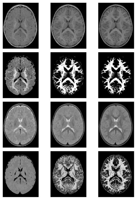
The clinical images are first corrected for intensity inhomogeneity and then co-registered using a nonlinear, free-form, spline-based deformation algorithm [11]. The earlier time point images of each subject are registered to the image of that same subject scanned at the latest time point. This is followed by constructing a common atlas space into which the entire image set is deformed using an unbiased atlas building procedure [12]. Once all the images are in the same coordinate space, they are then segmented into the major tissue classes using an atlas-moderated multi-modal Expectation-Maximization algorithm. The earlier time point images of each subject are segmented consistently by applying the segmentation map of the same subject at a later time point as a probabilistic prior. The generated intensity profiles are modeled as Gaussians and used for computation of subject specific tissue class probability maps. Fig. 1 shows the input images and the marginal probability maps for specific modalities.

Figure 1.

T1W (first row) and T2W (third row) MR images of a single subject and their corresponding T1W (second row) and T2W (fourth row) white matter probability maps, scanned approximately at ages 6, 12, and 24 months (from left to right).

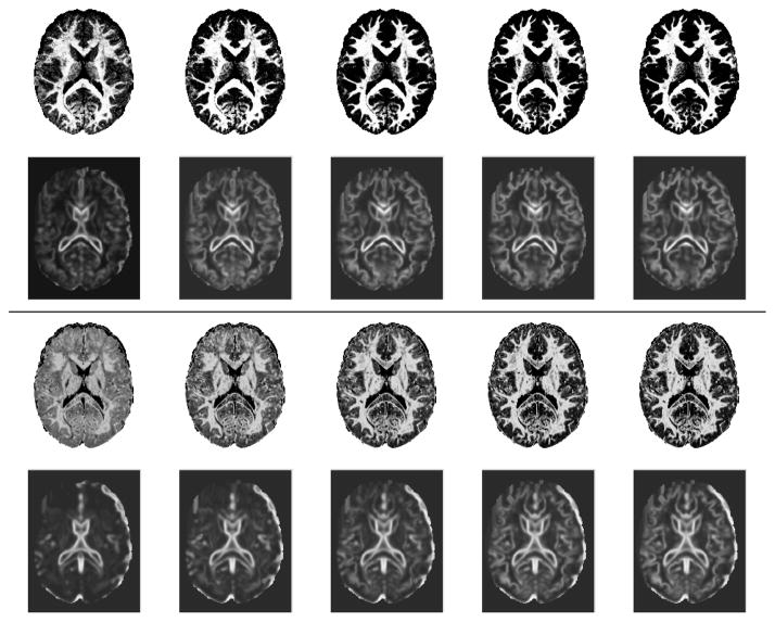
We interpolate the tissue probability maps using the combination of LogOdds mapping and kernel regression, where we apply a Gaussian kernel with standard deviation of 4 months. Fig. 2 shows the interpolated probability maps and corresponding contrast values at 9, 12, 15, 18, and 21 months of age, which we computed for a single 2D slice. We observe that the probability maps become less noisy and show clearer, better defined structures across time. It can be seen from the contrast maps that the boundaries between tissue classes also show higher contrast as time progresses. This effect is seen at an earlier stage in the T1W images and at a later stage in T2W images, confirming previous studies which show that these two modalities capture the initial and more advanced stages of the maturation process respectively.

Fig. 2.

Interpolated white matter probability maps of T1W (first row) and T2W (third row) of a single subject at ages 9, 12, 15, 18, and 21 months (from left to right) and their corresponding contrast maps (T1W-second row and T2W-fourth row).

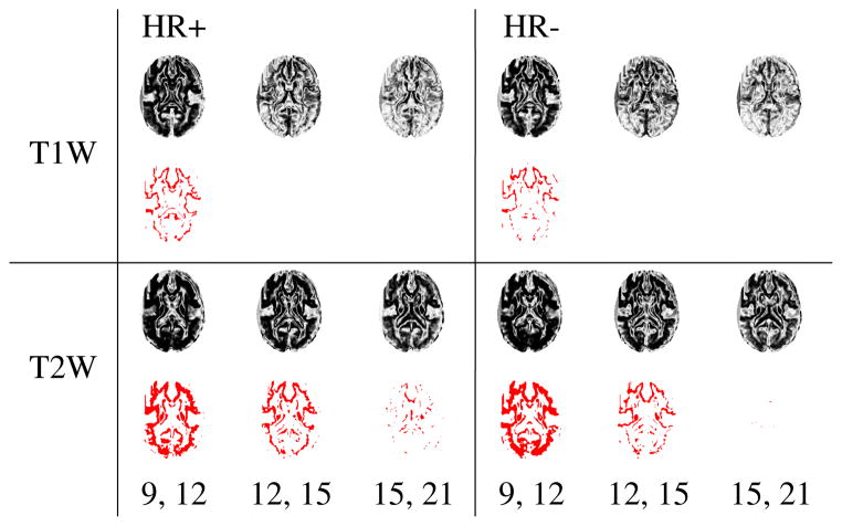
We conduct statistical tests based on the two-sample t-test, both among groups at specific time points and across time points in a specific group. Multiple comparison corrections are performed using the False Discovery Rate (FDR) algorithm at a level of 0.05. When comparing HR+ and HR− groups, we observe that the p-values show distinct trends across time (Fig. 3), although significance is not seen after corrections for multiple comparisons. When contrast maps from time points that were 6 months apart (for eg. 9 months and 15 months) were tested against each other, trends were seen in the p-values. We detect regions of significance even after corrections, as shown in Fig. 4. We note that these regions of significance shrink when later time points are studied, therefore indicating that the major changes in contrast take place during the first year after birth.

Fig. 3.

Comparison between the HR+ and HR− population groups, with p-values computed from contrast maps at time points 9, 12, 15, 18, and 22 months for T1W (first row) and T2W (second row) images.

Fig. 4.

Temporal comparison between time points in a specific group. First and third rows show the p-values computed on contrast maps between time points that are 6 months apart. Second and fourth rows show the corresponding significance maps. The first three columns show results for the HR+ group. The last three columns show results for the HR− group.

4. CONCLUSIONS

We propose a new method for quantitative analysis of early brain maturation by quantification and analysis of contrast at each voxel and across different time points. Our method uses regression in the LogOdds space and information theoretic measures of distance between distributions to capture contrast in a manner that is robust to imaging parameters and without requiring intensity normalization. We applied our method to a clinical neuroimaging study on early brain development, where we obtain a 4D spatiotemporal model of contrast changes in multimodal MRI. We did not observe significant differences across populations, likely due to the limited number of samples used in our experiment. We observed significant differences across time points in a population, where differences are more pronounced in the first year of development. In the future, we will conduct experiments on larger population sizes and we will explore the addition of other modalities such as diffusion tensor imaging that captures additional information on brain white matter development.

References

- 1.Rutherford Mary. MRI of the Neonatal Brain. W.B. Saunders; 2002. [Google Scholar]
- 2.Barkoyich J, Kjos B, Jackson D, Norman D. Normal Maturation of the Neonatal and Infant Brain: MR Imaging at 1.5 T. Radiology. 1988;166:173–180. doi: 10.1148/radiology.166.1.3336675. [DOI] [PubMed] [Google Scholar]
- 3.Giedd JN, Blumenthal J, Jeffries NO, Castellanos FX, Liu H, Zijdenbos A, Paus T, Evans AC, Rapoport JL. Brain development during childhood and adolescence: a longitudinal MRI study. Nat Neurosci. 1999 Oct;2 doi: 10.1038/13158. [DOI] [PubMed] [Google Scholar]
- 4.Prastawa M, Sadeghi N, Gilmore JH, Lin W, Gerig G. A new framework for analyzing white matter maturation in early brain development. Proc ISBI. 2010:97–100. doi: 10.1109/isbi.2010.5490404. [DOI] [PMC free article] [PubMed] [Google Scholar]
- 5.Serag A, Aljabar P, Counsell S, Boardman JP, Hajnal JV, Rueckert D. Tracking developmental changes in subcortical structures of the preterm brain using multi-modal MRI. ISBI. 2011:349–352. [Google Scholar]
- 6.Davatzikos C, Resnick SM. Degenerative age changes in white matter connectivity visualized in vivo using magnetic resonance imaging. Cerebral Cortex. 2002;12(7):767–771. doi: 10.1093/cercor/12.7.767. [DOI] [PubMed] [Google Scholar]
- 7.Vardhan A, Prastawa M, Gouttard S, Piven J, Gerig G. Quantifying regional growth patterns through longitudinal analysis of distances between multimodal mr intensity distributions. Proc ISBI. 2012 doi: 10.1109/isbi.2012.6235765. [DOI] [PMC free article] [PubMed] [Google Scholar]
- 8.Pohl KM, Fisher J, Bouix S, Shenton ME, McCarley RW, Grimson WEL, Kikinis R, Wells WM. Using the Logarithm of Odds to Define a Vector Space on Probabilistic Atlases. Medical Image Analysis. 2007;11(6):465–477. doi: 10.1016/j.media.2007.06.003. [DOI] [PMC free article] [PubMed] [Google Scholar]
- 9.Habas P, Kim K, Corbett-Detig JM, Rousseau F, Glenn OA, Barkovich AJ, Studholme C. A spatiotemporal atlas of MR intensity, tissue probability and shape of the fetal brain with application to segmentation. NeuroImage. 2010;53:460–470. doi: 10.1016/j.neuroimage.2010.06.054. [DOI] [PMC free article] [PubMed] [Google Scholar]
- 10.Genovese CR, Lazar N, Nichols TE. Thresholding of statistical maps in functional neuroimaging using the false discovery rate. NeuroImage. 2002:870–878. doi: 10.1006/nimg.2001.1037. [DOI] [PubMed] [Google Scholar]
- 11.Rueckert D, Sonoda LI, Hayes C, Hill DL, Leach MO, Hawkes DJ. Nonrigid registration using free-form deformations: application to breast MR images. IEEE TMI. 1999 Aug;18:712–721. doi: 10.1109/42.796284. [DOI] [PubMed] [Google Scholar]
- 12.Joshi S, Davis B, Jomier M, Gerig G, et al. Unbiased diffeomorphic atlas construction for computational anatomy. NeuroImage. 2004;23(1):151. doi: 10.1016/j.neuroimage.2004.07.068. [DOI] [PubMed] [Google Scholar]