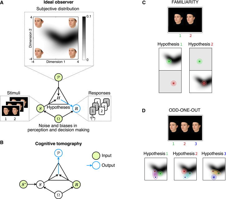
Figure 1.

Cognitive Tomography Applied to Estimating Priors for Faces

(A) Information flow in the ideal observer model. In the model, a subjective distribution, $\mathcal{P}$, encodes prior knowledge about stimuli. In this study, a subjective distribution for faces assigns a probability value (gray levels) to each face as a function of its location in feature space (here the two dimensions of the feature space correspond to the first two principal components of the structure of faces [19] and are measured in units of SD). Representative faces corresponding to the corners of the feature space are shown. The ideal observer infers hypotheses, H, about the stimuli it perceives, S, using prior knowledge encoded in $\mathcal{P}$. Based on the inferred hypotheses, it computes the final response R. Both perception and decision making are subject to noise and biases, $\Omega$.

(B) Cognitive tomography inverts the ideal observer model to compute $\mathcal{P}$ based on R and the presented stimuli, S^∗, which is corrupted by perceptual noise to yield S. Note that information available to the ideal observer and cognitive tomography (circles with green fill) to compute their final output (blue arrows and circles) is complementary.

(C) In the familiarity task, participants are presented with a pair of faces (top) and are required to pick the one that they judge more familiar. Each face corresponds to a particular location in feature space (colored dots in the bottom panels correspond to stimuli in the top panels). The ideal observer model makes its choice by considering two hypotheses (bottom; hypothesis 1, face 1 is more familiar than face 2; hypothesis 2, vice versa) that each specify a way in which the stimuli could have been generated. According to these hypotheses, the familiar face is a sample from the subjective distribution (corrupted by perceptual noise; colored covariance ellipses), and the unfamiliar face is sampled randomly and uniformly from the feature space (also subject to perceptual noise). Given a subjective distribution and the covariance of perceptual noise, the ideal observer assigns a probability to each hypothesis and then through a decision process (also including noise) determines the probability of each possible response.

(D) In the odd-one-out task, participants are presented with three faces and are required to pick the one that looks the most different from the other two (top). Each hypothesis corresponds to two of the faces being noise-corrupted versions (bottom; pairs of dots enclosed by covariance ellipses) of the same underlying face (centers of ellipses) and the third face (the odd one out) being a noisy version of a truly different face (isolated dots within covariance ellipses, here shown as circles).

See also Figure S1 for further details and validation of the method.