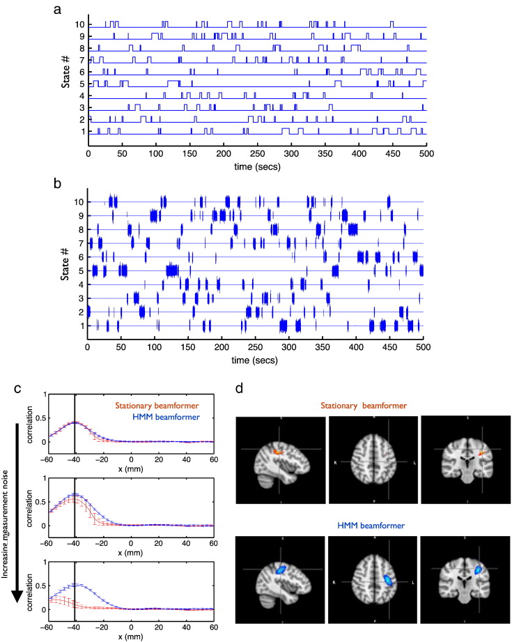
Fig. 1.

Example of data simulated to contain time-varying “confound” sources using a 10 state HMM. The resulting HMM state time courses are shown in (a), and the resulting simulated signals (in brain space) are shown in (b). These “confound” sources are placed at the MNI coordinates listed in Table 1, along with a unit variance Gaussian random “signal” source (not shown) placed in the left motor cortex (LMC) to create simulated MEG data. Comparisons of standard stationary beamformer (red) and HMM beamformer (blue) using the simulated data. (c) Correlation over time (and over all states) between the beta-band power time courses of the beamformed data and the known signal in the LMC, as x is varied while fixing y = − 25 mm and z = 49 mm with different amounts of sensor measurement noise. Error bars show standard deviation over 10 realisations. (d) T-statistic maps of the correlation with the known beta-band power time course for a single realisation of the simulated data at the highest measurement noise, thresholded at the 99th percentile; the cross hairs are at the true location of the signal.