Figure 6.

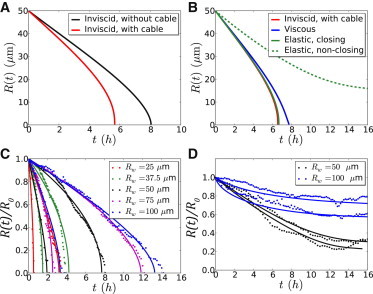
Trajectories. Model predictions: Plots of individual trajectories of the wound radius R(t), R₀ = 50 μm. (A) Contribution of border forces for an inviscid fluid. Plots of R(t) as given by Eq. S11, D = 200 μm² h⁻¹, R_max = 110 μm (without cable, black curve); and Eq. S10, with the same values of D and R_max, R_γ = 10 μm (with cable, red curve). (B) Rheology. Plots of R(t) as given by Eq. S10 (inviscid liquid, as in A (red curve)); Eqs. S16 and S17, with R_η = 10 μm (blue curve, viscous liquid); Eqs. S23 and S24, with $2\mu /{\sigma }_{\text{p}}=0.1$ (solid green curve, elastic solid, closing); Eq. S26, with R_e = 15 μm (elastic solid, nonclosing, dashed green curve,); The values of D, R_max, and R_γ are the same as in A. Experimental data and fits (C) Normalized effective radius, R(t)/R₀, is plotted as a function of time t for MDCK wild-type wounds. For clarity, we show only two trajectories (circles) and their fits by Eq. S11 (solid curves) per pillar size, R_w, corresponding to the shortest and longest closure time observed at a given R_w. (D) Normalized effective radius, R(t)/R₀, is plotted as a function of time t for nonclosing wounds of the MDCK Rac⁻ assay. For illustrative purposes, we show only two trajectories t(R) per pillar size R_w (solid curves) and their fit by Eq. S26 (dashed curves), with the constraints D_s ≥ 0, R_max ∈ [96,114] μm (confidence interval obtained from closure-time data) and R_e = min R(t). Note that (Eq. S26) is defined only for R > R_e.