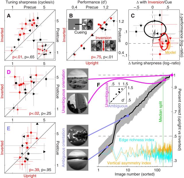
Figure 3.

Tuning sharpness is affected by image inversion. Red symbols in A plot sharpness (Fig. 1H) for inverted (y-axis) versus upright (x-axis) trials, black symbols for postcue (y-axis) versus precue (x-axis) trials. A, Inset plots sharpness as estimated via fitting (smooth traces in Fig. 1G; see Materials and Methods for details). B, Plots sensitivity using similar conventions. C, Plots the log-ratio change in sensitivity (y-axis) versus the change in tuning sharpness (x-axis) for both inversion (red) and spatial cueing (black). Ovals are centered on mean values with radius matched to SD along the corresponding dimension; arrows point from origin to mean coordinates. Orange shading shows range spanned by top-down predictive model (Fig. 4, see Materials and Methods). D, E, Plot same as A, but after splitting the dataset into images with unambiguous versus ambiguous orientation (respectively). Images were assigned to either category based on the associated aggregate performance for discriminating upright versus inverted configuration (y-axis in F) of individual images (x-axis): those above the median performance value (vertical green line) were assigned to the unambiguous category, those below to the ambiguous one (see Materials and Methods for experimental details). Orange/cyan traces plot two image-based metrics (arbitrarily rescaled along y-axis) quantifying vertical asymmetry and edge richness of individual images (see Materials and Methods). Inset plots sensitivity for performing the probe discrimination task with unambiguous versus ambiguous scenes. F, Left, Examples of images from the two categories. Different symbols refer to different observers. Error bars indicate ± 1 SEM (not visible when smaller than symbol). p values show the result of paired two-tailed Wilcoxon signed rank tests for the comparison between values on the y-axis versus corresponding values on the x-axis.