Figure 8.

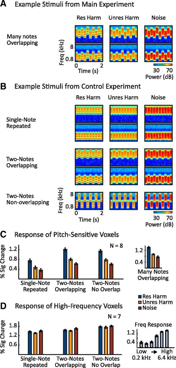
Effect of frequency variation on cortical responses to resolved and unresolved harmonics. A, Cochleograms for example resolved (left, harmonics 3–6), unresolved (middle, harmonics 15–30), and noise (right) stimuli from the main experiment. Each stimulus was composed of several different notes with overlapping frequency ranges. Low- (bottom) and high- (top) frequency examples are shown for each note type. Cochleograms were computed as in Figure 2B. B, Cochleograms illustrating the 3 × 3 factorial design used in the control experiment. Stimuli were composed of a single repeated note (top row), two alternating notes with overlapping frequency ranges (middle row), or alternating notes with nonoverlapping frequency ranges (bottom row). Each note was composed of resolved harmonics (left column, harmonics 3–6), unresolved harmonics (middle column, harmonics 15–30), or noise (right column). All conditions spanned a frequency range similar to that of the stimuli in the main experiment. C, Response of pitch-sensitive voxels to the nine conditions of the control experiment. Pitch-sensitive voxels were identified by contrasting resolved harmonics with noise using the stimuli from the main experiment (illustrated in A). The inset shows responses to the analogous resolved harmonics, unresolved harmonics, and noise conditions from the main experiment (measured in data independent of the localizer). D, Response of high-frequency-preferring voxels to the nine conditions of the control experiment. High-frequency voxels were identified by contrasting high- (1.6, 3.2, 6.4 kHz) and low- (0.2, 0.4, 0.8 kHz) frequency pure tones. The inset shows responses to the six pure-tone conditions used to localize the region (measured in data independent of the localizer). Error bars indicate one within-subject SEM.