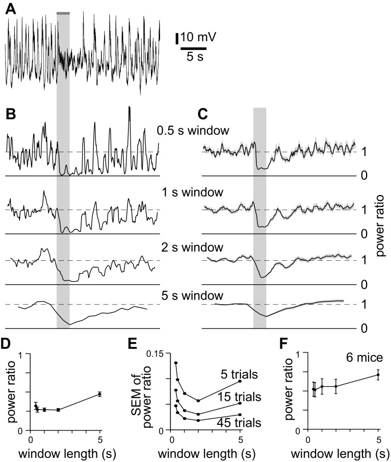
Fig. 3.
Analysis of low-frequency power. A: example of a LFP recording. Bars and gray shaded areas indicate illumination of the cortical surface with fifty 10-ms light pulses at 20 Hz, starting at 10 s. B: power ratio for the recording in A, calculated using different window lengths. Power was normalized to that 2–10 s before stimulus onset. For each plot, y-axis represents normalized power; solid horizontal line is at 0; dashed horizontal line at 1. Time scale aligned to A. Bandwidths: 0.375-s window, 5.86 Hz; 0.5-s window, 3.9–5.86 Hz; 1-s window, 1.95–5.86 Hz; 2-s window, 0.9766–5.86 Hz; 5-s window, 0.4883–5.86 Hz. C: mean power ratio from 45 trials, for the mouse in A–C, calculated using different window lengths. Shading denotes ±SE. D: comparison of power ratio for different window lengths, for 45 trials from the same mouse as A–D. E: comparison of trial-to-trial variability (SE of normalized power) for different window lengths, for 45 trials from the same mouse as A–E. F: power ratio as a function of window length. Each point represents means ± SE of 45 trials in each of 9 mice.

