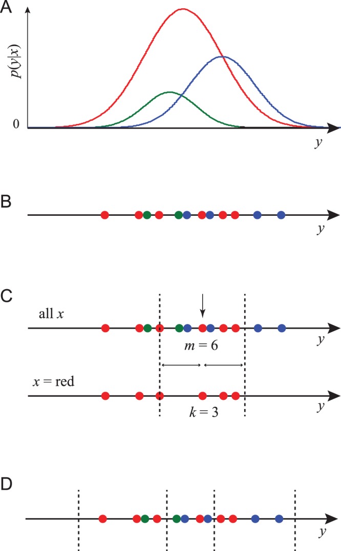
Figure 1. Procedures for estimating MI.

(A) An example joint probability density  where
where  is a real-valued scalar and
  can take one of three values, indicated red, blue and green. For each value of
  the probability density in
  is shown as plot of that color, whose area is proportional to
  . (B) A set of
  data pairs sampled from this distribution, where
  is represented by the color of each point and
  by its position on the
  -axis. (C) The computation of
  in our nearest-neighbor method. Data point
  is the red dot indicated by a vertical arrow. The full data set is on the upper line, and the subset of all red data points is on the lower line. We find that the data point which is the 3rd-closest neighbor to
  on the bottom line is the 6th-closest neighbor on the top line. Dashed lines show the distance
  from point
  out to the 3rd neighbor.
  ,
,  , and for this point
  and
and  . (D) A binning of the data into equal bins containing
  data points. MI can be estimated from the numbers of points of each color in each bin.
