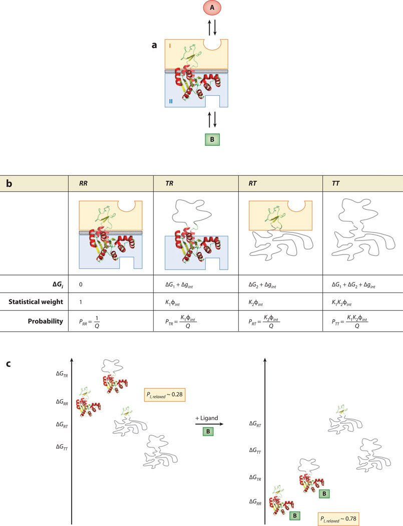
Figure 3.

The ensemble allosteric model (EAM) applied to a two-domain allosteric protein. (a) Schematic representation of a hypothetical two-domain allosteric protein. Domain I (orange box) binds ligand A, and domain II (blue box) binds ligand B. The diagonal-striped area depicts a specific interaction between the two folded domains (i.e., R states) with a free energy Δg_int. Note that this system is conceptually identical to the protein ensemble depicted in Figure 1c. (b) Boltzmann-weighted populations of each microstate in the ensemble. R, relaxed, or high-affinity, state; T, tense, or low-affinity, state. Although the cartoons for T domains appear unstructured, all equations apply equally well to the case in which both T and R states are structured but exhibit a difference in binding affinity. (c) A specific case demonstrating allosteric coupling: Stabilizing domain II with ligand B also stabilizes domain I owing to the favorable interaction energy. Site-to-site coupling is evaluated through the addition of ligand B. Because addition of ligand B stabilizes those states that bind ligand B, the ensemble probabilities are redistributed. Binding of ligand at site B is thus coupled to the transition of domain I from a T state to a R state (possibly but not necessarily folding of domain I) as described in the text. The biologically reasonable values used for this example are ΔG₁ = −0.7 kcal mol⁻¹, ΔG₂ = −2.3 kcal mol⁻¹, Δg_int = +1.6 kcal mol⁻¹, Δg_Lig,B = −3.0 kcal mol⁻¹.