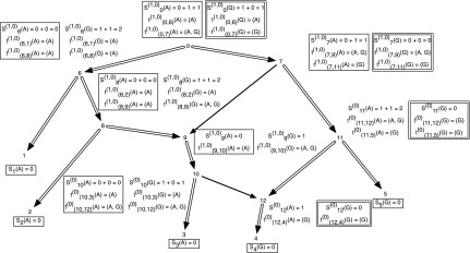
FIG. 2.

An example showing one among the at-most two dimensions of storage at each vertex of a phylogenetic network for computing the softwired score and all optimal assignments on the network. The costs of each state at each node are shown next to the corresponding vertex; the cost matrix considered here is given by cij = 1 if i ≠ j and 0 if i = j for the states  . We order the reticulate vertices as (9, 12). The superscript (0) in Sv(.) at the vertices v = 10, 11, and 12 corresponds to the state 0 at the vertex 12, which in turn corresponds to the deletion of the left edge (10, 12) incident at vertex 12 and the superscript (1, 0) in Sv(.) at the vertices v = 0, 6, 7, 8, and 9 corresponds to the states at the reticulate vertices 9 and 12 respectively, corresponding to the deletion of the right edge (7, 9) incident at vertex 9 and the left edge (11, 12) incident at vertex 12. Note that there are exactly three optimal assignments corresponding to the superscript (1, 0), namely α1(.), α2(.) and α3(.) given by α1(1) = A, α1(2) = A, α1(3) = A, α1(4) = G, α1(12) = G, α1(10) = A, α1(9) = A, α1(8) = A, α1(6) = A, α1(5) = G, α1(11) = G, α1(7) = G, α1(0) = G; α2(1) = A, α2(2) = A, α2(3) = A, α2(4) = G, α2(12) = G, α2(10) = A, α2(9) = A, α2(8) = A, α2(6) = A, α2(5) = G, α2(11) = G, α2(7) = G, α2(0) = A and α3(1) = A, α3(2) = A, α3(3) = A, α3(4) = G, α3(12) = G, α3(10) = A, α3(9) = A, α3(8) = A, α3(6) = A, α3(5) = G, α3(11) = G, α3(7) = A, α3(0) = A. These assignments can be obtained by preorder traversal of the spanning tree in N (whose edges are shown in double arcs) obtained by deleting the edges (7, 9) and (11, 12). The optimal assignments and its corresponding storage entries at each vertex are highlighted in boxes. Note that both the character states A and G are attained at the root vertex 0.
