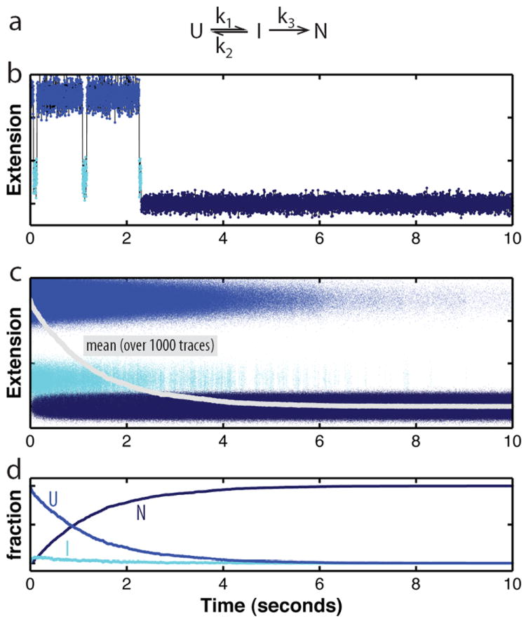
Figure 4. Stochasticity of folding.

a. Kinetic scheme for a folding reaction consisting of the reversible population of a folding intermediate (I) from the unfolded state (U) prior to folding to the native state (N). I is an obligate, on-pathway intermediate in this scheme. b. Simulated folding trajectory based on the kinetic mechanism in panel a. A molecule hops between the unfolded and an intermediate state before irreversibly folding to the native state, governed by the rate constants indicated in the kinetic scheme. The changes in molecular extension, which can be measured with optical tweezers, reflect transitions between the states. In this single trace, the population of the folding intermediate is easily discernible. Because the dwell times in the individual states are exponentially distributed around the mean (which equals 1/k), the number of transitions between U and I are variable, as is the time required to reach the native state. c. Overlay of 1000 folding trajectories simulated based on the kinetic scheme given in panel a (parameters : k₁ = 2.5 s^-1, k₂ = 20 s^-1, k₃ = 10 s^-1). Even though folding proceeds according to the same rate constants and is initiated at the same time for all traces, the time for folding to the native state varies greatly among the traces. The average (grey line) was reconstructed from the individual traces, but the features of the individual traces cannot be recovered from the average. d. Evolution of the three folding states over time. The plot shows the relative amounts of U, I, and N over time, calculated from the data in panel c.