Figure 4.

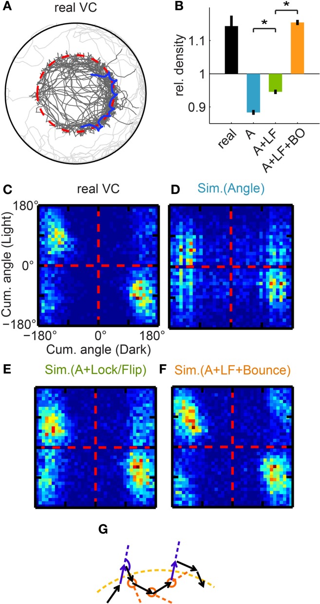
Affinity to the virtual border. (A) Trajectory of a real fish, example trajectory segment highlighted in blue. Note that the trajectory density is much higher close to the virtual border (dotted red line). (B) Quantification of the relative bout density close to the virtual border, and comparison between real fish and different simulations. Simulations are labeled by the algorithms implemented: “A” = Algorithm I [Angle], “LF” = Algorithm II [Lock/Flip], “BO” = Algorithm III [Bounce]. Reference level (=1) is the normalized baseline bout density if the trajectory were uniformly distributed within the Virtual Circle. (Quantification see Figure S4A) (C–F) Correlation between the cumulative angle turned during a light interval and during the preceding dark interval, again shown by matrices as in Figure 3B. (C) For real fish, strong clustering is shown close to the “flip” diagonal. (D) For the simulation with Algorithm I [Angle], there is no strong “lock”/“flip” bias. (E) In the simulation including Algorithm II [Lock/Flip], clustering in the “lock” quadrants is stronger than for real fish. (F) In the simulation including Algorithm III [Bounce], the simulated fish are constrained to match the “flip” pattern of real fish, and the resulting matrix confirms that the similarity to real fish is achieved. As shown in the last bar of (B), the addition of this algorithm restores the high bout density of real fish in the simulation. (G) Illustration of Algorithm III [Bounce]. If the fish exits the virtual border at approximately the same angle (relative to the border) each time, the fish may frequently cross the virtual border. That would require the heading direction of the two purple bouts to be approximately parallel, and the angle of the turn in dark (marked with the purple arc) should have equal magnitude but opposite direction as the sum of the 3 following turns in light (marked with orange circles). ^*p < 0.001.