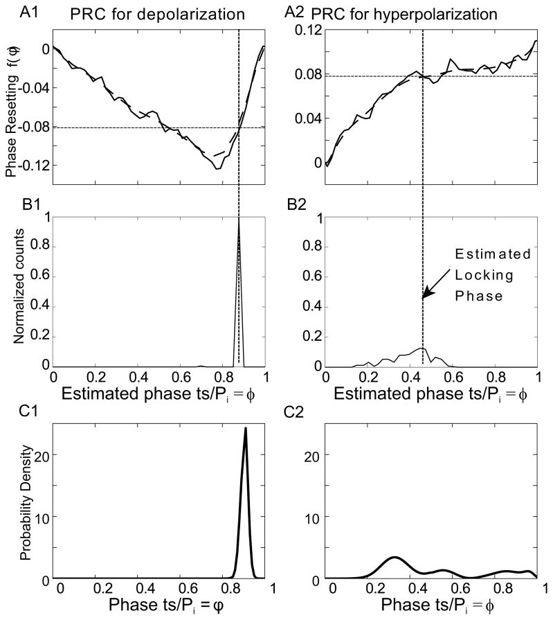
Figure 4.
Comparison of experimental and theoretical distribution of the phase at which the forcing stimulus arrives within the cycle of the forced neuron. A. Averaged PRC (solid line) for CA1 pyramidal neurons (n=14). Data from Wang et al 2013. Data was smoothed by fitting to a Bezier polynomial function (thick dashed curve). A1) PRC for depolarizing pulse, A2) PRC for hyperpolarizing pulse. The thin dashed horizontal line in A1 and A2 corresponds to deterministic value of f(φ*) for the mean period computed using Eq. 9. B. Phase distribution for one representative example. B1) Depolarizing pulse train: PF=100ms, Pi=134.12 ± 8.79424 ms, B2) Hyperpolarizing pulse train: PF=102.6, Pi=99.4±7.6 ms. C. Probability density calculated using Eq. 11. C1) Using the PRC from A1 with parameters : PF=100 ms and Pi=106±1.5ms and C2) Using the PRC in A2 and parameters PF=102ms and Pi=95±1.5ms. Since the PRCs in A and the distributions in B are from different studies, the correspondence between theory and experiment is only qualitative.

