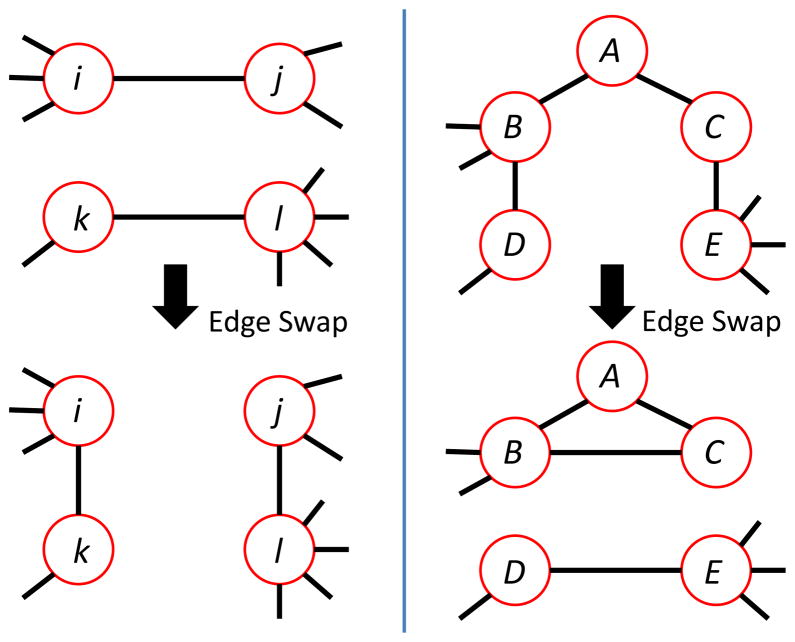
FIG. 8.

(Color online) A degree distribution-preserving edge swap. The four vertices shown are connected by the edge stubs shown here to the rest of the graph, which is not shown. (left panel) Assortativity-changing edge swap: In this example, d_i = 4, d_j = 3, d_k = 2, and d_l = 5. Hence d_id_j +d_kd_l = 22 and d_id_k + d_j d_l = 23 so the graph at the bottom has a higher assortativity than the one at the top [29, 30]. If the graph at the top is connected, the graph at the bottom will also be connected if there is a path from i to j. In that case, this will be an acceptable edge swap for A⁺, but not for A⁻. (right panel) Assortativity-preserving and triangle-changing edge swap: B and D have no neighbors in common, nor do C and E. In this example, d_B = d_E = 4 and d_C = d_D = 2. Hence d_Bd_D + d_C d_E = 40 = d_Bd_C + d_Dd_E so the graph at the top has the same assortativity as the one at the bottom. If the graph at the top is connected, the graph at the bottom will also be connected if there is a path from B to D. In that case, the swap from top configuration to bottom configuration will be an acceptable one for T⁺; the swap in the opposite direction will be acceptable for T⁻, since the swap cannot disconnect the graph. This swap changes the number of triangles in the graph by at least one – more, if B and C have any common neighbors besides A.