Figure 1.

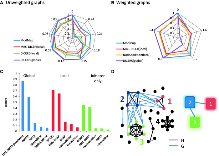
Module map: example and simulation results. (A and B) Performance of module map algorithms on 500-node graphs. (A) Unweighted graphs. (B) Weighted graphs. Each simulated pair of graphs contained an embedded module map of six modules in a tree structure. In addition, two random cliques and two bicliques were embedded in the graphs as decoys. Module, clique and biclique size was chosen uniformly at random between 10 and 20. In the unweighted model (A) each edge was replaced by a non-edge with probability P and vice versa. In the weighted model (B) edge weights are sampled from the normal distribution N(1,σ), and non-edge weights are sampled from the normal distribution N(−1, σ). Results are averages of 10 simulations for each data point. The four top performing algorithms for each simulation are presented using radar plots. MBC-DICER with global improvement is denoted as ModMap. The Jaccard coefficient between the modules produced by each algorithm and the true modules is shown as the distance from the center. Consecutive spokes from the top anticlockwise show increasing values of P in A and of σ in B. (C) Comparison of module map algorithms on unweighted graphs with 1000 nodes, containing a map of 10 modules and five decoys and P = 0.15. (D) A toy example of the module map problem; left: the two networks. Nodes are genes, H edges are black and G edges are blue; right: the module map. Nodes are modules and edges are links. Colors and numbers are the same on the left and right. The map contains three modules: module 2 is linked to modules 1 and 3, whereas module 1 and 3 are not linked. Black nodes are not part of the module map. The graph H (black edges) contains a clique that is not linked in G to another module and thus is not a part of the map. The example also demonstrates the difference between the local and global approaches. The local approach identifies modules 1 and 2 as linked, whereas the global approach also identifies module 3 as linked to module 2. See text.