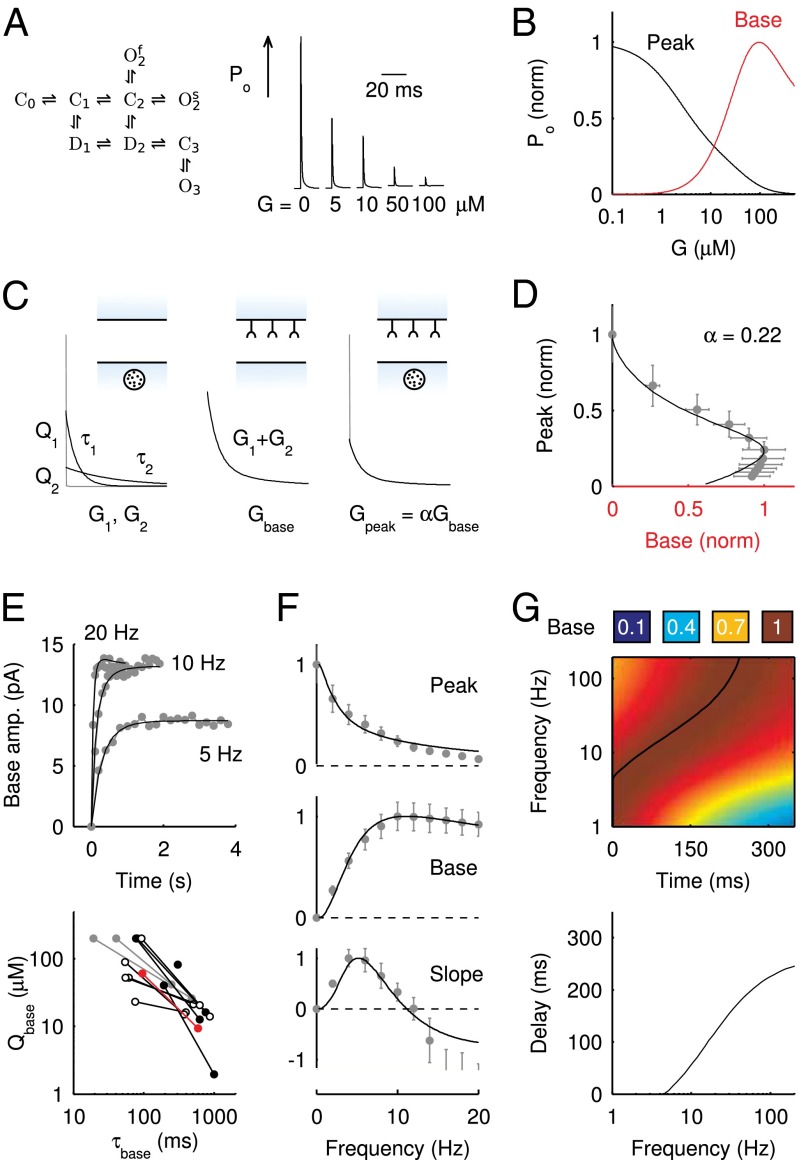
Fig. 4.
AMPAR model simulations. (A) Schematic representation of the AMPAR model from Raman and Trussell (2). Traces are simulation results of total (summed) receptor open probability Po in response to a 4-mM pulse of glutamate for five values of the ambient glutamate concentration G. (B) Peak Po
 in response to a brief 4-mM glutamate pulse (black trace) as a function of G. The steady-state Po
 as a function of G is plotted in red. (C) Glutamate release and decay model. The background glutamate concentration G was modeled as an instantaneously released quantity, which decayed biexponentially to zero (black). The gray curves represent the fast glutamate peak (truncated) underlying the fast EPSC. Further details are described in the main text. (D)
  as a function of
  (black curve). The steady-state AMPAR model was fitted to experimental steady-state data (gray) with fit parameter α. (E) Results of fitting the biexponential glutamate decay model to EPSC base amplitudes obtained from regular stimulation experiments (Upper). Each fit was characterized by a pair of release amplitudes
  and decay time constants
  ; results are shown in the bottom panel for 11 UBCs. (F) Model fit to steady-state data of Fig. 2. Fit results are shown in red in E. (G) (Upper)
  as a function of time following 10 regular stimuli at varying stimulation frequency. The black curve denotes the time of maximal
  . (Lower) Delay of the maximal
  as a function of stimulation frequency for 10 stimuli.

