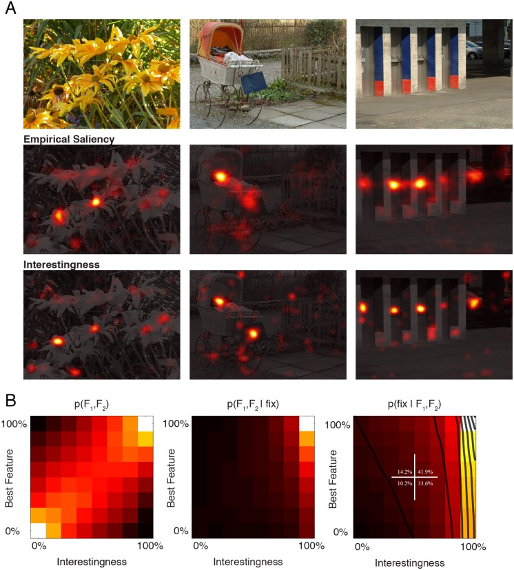
Figure 7. Computation of Interestingness maps.

(A) 3 different stimuli are shown together with their actual fixation and interestingness maps (second and third rows). The first row depicts three stimuli belonging to Natural and Urban categories as they were shown during the experiment. Second and third rows depict the empirical saliency and interestingness maps overlaid on the gray scale version of the stimulus. Empirical saliency maps are probability maps that show the probability of a given location to be fixated. Similarly interestingness maps represent for a given location the probability of receiving an interestingness rating. These were obtained with the help of a pointer device by an independent set of human subjects (n = 35). These maps were treated the same way as low-level feature maps in order to compute D_KL values. (B) Joint distribution of interestingness values and a low-level feature (Cornerness) that was most strongly correlated with fixation locations (Left panel). This distribution shows the co-occurrence of a low-level image based feature with interestingness ratings of human subjects at all fixated and non-fixated locations. Middle panel represents the distribution of same variables at exclusively fixated locations. The posterior distribution represents the two-dimensional saliency function (right panel). Notice that the saliency increases nearly completely as a function of interestingness ratings (contour lines) and only marginally as a function of low-level feature values. The saliency is therefore mainly modulated by the interestingness value of a location.