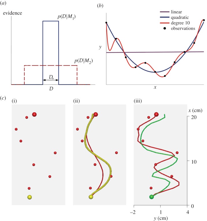
Figure 1.

Bayesian Occam's Razor. (a) Schematic plot of evidence for a simple model M₁ (blue, solid line) and a complex model M₂ (red, dashed line) for different data such as different random trajectories. Because both models have to spread unit probability mass over all compatible observations, the simpler model M₁ has a higher evidence in the overlapping region (b) Exemplary polynomials of different degrees fitted to noisy observations (black dots) by minimizing mean-squared error. The linear model (purple line) is not flexible enough to capture the underlying function and results in a large fitting error. The most complex model (red line) is too flexible and passes exactly through each data point, thus achieving a fitting error of zero. A reasonable fit should trade off the complexity of the model against the goodness of fit. In this example, this is achieved by the quadratic model (blue line). (c) Standard trials. (i) Noisy observations are shown to the participant as small red spheres. Start position (yellow sphere) and end position (larger red sphere) are noise-free. The yellow colour of the start sphere indicates that the underlying trajectory was drawn from M₁ with the long length scale. (ii) After completion of a standard trial, the underlying trajectory (red) is revealed and shown along with the participants trajectory (yellow). (iii) Example of a standard trial where the short-length-scale model M₂ was the generating model, as indicated by the green colour of the start position and participants trajectory. Note that the noisy observations are exactly the same in all three panels and the drawn trajectories were recorded from the same participant.