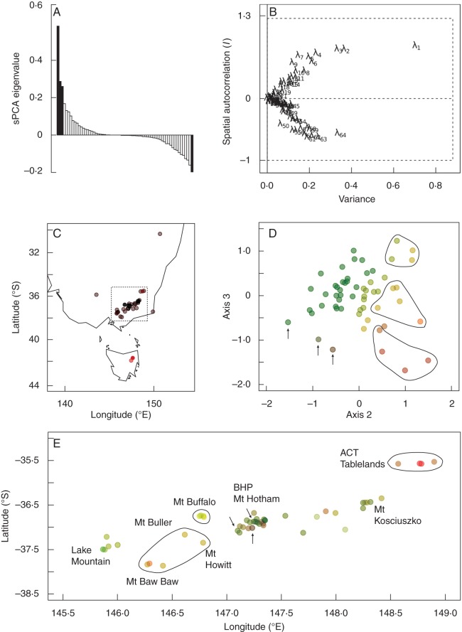
Fig. 2.

sPCA results for the microsatellite data set revealing spatial genetic structure across species boundaries. (A) sPCA eigenvalues. Positive eigenvalues reflect global patterns and negative eigenvalues reflect local patterns. Eigenvalues retained in the final model are highlighted in black. (B) Screeplot of sPCA eigenvalues showing their decomposition into variance and spatial autocorrelation (Moran's I) components. λ₁, λ₂ and λ₃ are the first three positive eigenvalues from (A); λ₆₄ is the largest negative eigenvalue. These four eigenvalues were retained in the final model. (C) Axis 1 eigenvector sample scores (represented by colour on a black to red scale) plotted on the geographic locations, revealing Tasmania–mainland differentiation. The dotted box outlines the mainland area presented in (E). (D) Axis 3 vs. Axis 2 sPCA eigenvectors. Points are coloured-coded according to their positions along both axes. (E) Geographic location of mainland samples coloured by Axis 2 and 3 sPCA eigenvector score (see D for colour scheme). Geographic regions showing some distinctiveness in eigenvector space are circled. Points with similar, outlying eigenvector scores but no overall distinctiveness of geographic region are indicated by arrows. BHP, Bogong High Plains.