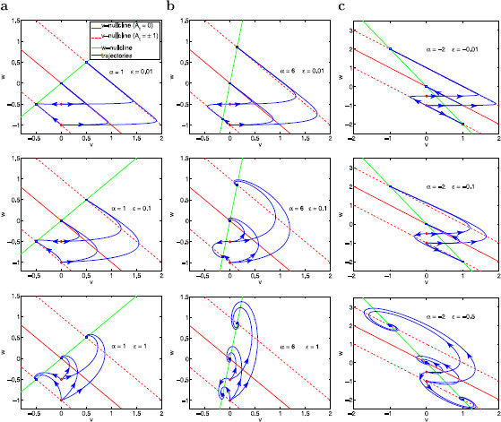
Fig. 4.

Phase-plane diagrams for the autonomous linear system (29)–(30) for various representative values of α, ϵ and $A_t$. a$\alpha =1$. Top row: $ϵ=0.01$. Middle row: $ϵ=0.1$. Bottom row: $ϵ=1$. b$\alpha =6$. Top row: $ϵ=0.01$. Middle row: $ϵ=0.1$. Bottom row: $ϵ=1$. c$\alpha =-2$. Top row: $ϵ=-0.01$. Middle row: $ϵ=-0.1$. Bottom row: $ϵ=-0.5$. Each panel shows superimposed phase-planes diagrams for three different constant values of $A_t$ ($=0,1,-1$) generating three v-nullclines (solid-red for $A_t=0$, dashed-red for $A_t=1$ and $A_t=-1$) and three fixed points (blue dots on the intersections between the red and green lines). The w-nullcline (green line) is common to all values of $A_t$. Solid-red line: v-nullclines for $A_t=0$. Dashed-red lines: v-nullclines for $A_t=1$ (above) and $A_t=-1$ (below). Red dots at $(0,-1)$ and $(0,-0.5)$: representative initial conditions. Solid-blue lines: trajectories initially located at these initial points. Each trajectory emerging from the red dots corresponds to a different value of $A_t$ and converges to the corresponding fixed point. The fixed points in panels a-top, a-middle and b-top are stable nodes and the fixed points in panels a-bottom, b-middle and b-bottom are stable foci