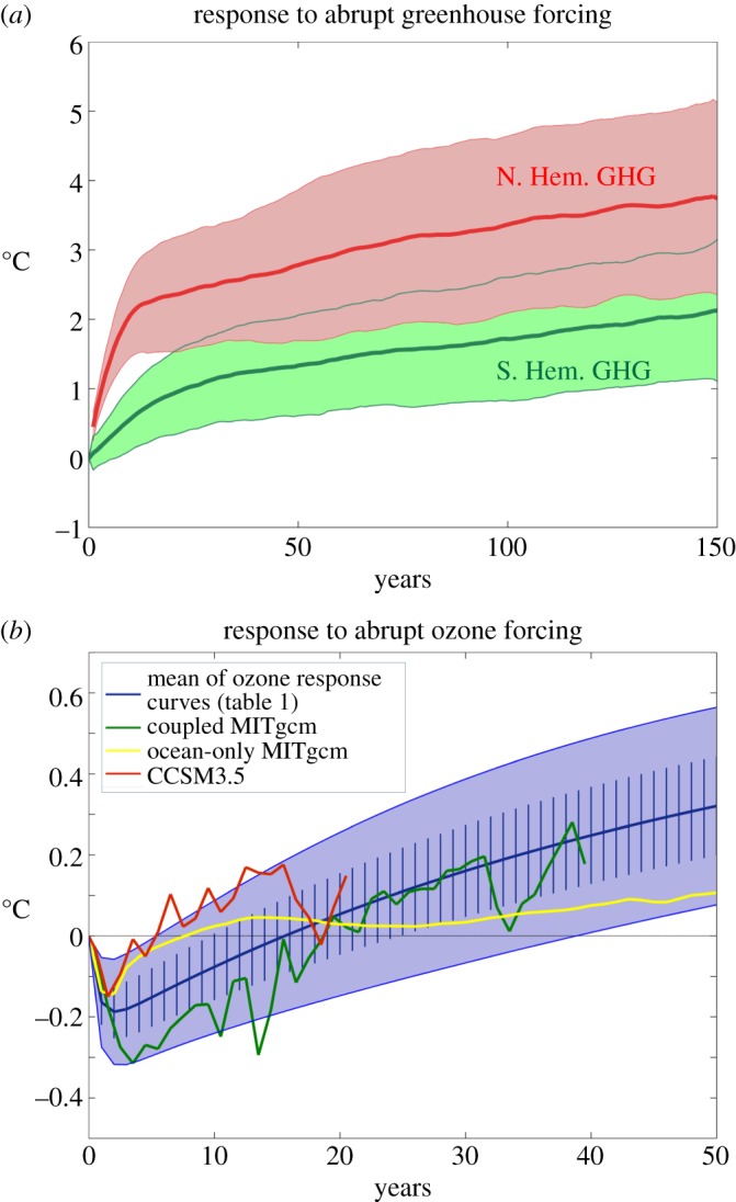
Figure 3.

Sea-surface temperature CRFs for: (a) GHG forcing computed from an ensemble of 15 CMIP5 models under quadrupling of CO₂. The Arctic is defined as north of 50° N (in red) and the Antarctic between 50° S and 70° S (in green). Thick lines denote the ensemble mean and the shaded area spans 1 s.d.; (b) ozone-hole CRFs based on the analytical expression equation (4.2) appropriate for a repeating annual cycle of amplitude approximately 100 DU. The thick blue line is the ensemble mean of the analytical response curves (table 1). Vertical hash marks represent 1 s.d., and the solid blue shading spans two standard deviations. The green curve is the ensemble mean SST response between 50° S and 70° S from abrupt ozone depletion experiments with the coupled MITgcm. The red curve shows the ensemble-mean evolution of the ‘cold pole’ of the SST dipole induced by abrupt ozone-hole forcing in the CCSM3.5 NCAR model from [39]. The yellow curve is the SST response between 50° S and 70° S from an abrupt SAM perturbation experiment with the ocean-only version of the MITgcm described in §3.