
Fig. 3.
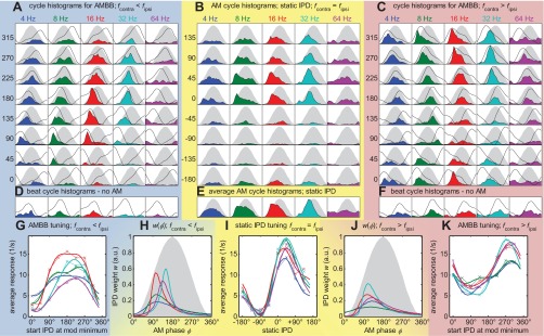
Response overview of inferior colliculus (IC) neuron #47; characteristic frequency (CF) = 320 Hz; 10 repetitions. All panels with blue backgrounds (left) belong to beating stimuli, with fcontra < fipsi; those with yellow backgrounds (middle) to AM tones with static IPDs; and those with red backgrounds (right) to beats, with fcontra > fipsi. A and C: latency-corrected cycle histograms (colored areas) for the 2 different beat directions of the AMBB. The 5 different columns of each panel represent different modulation (mod) frequencies (4, 8, 16, 32, and 64 Hz, from left to right). The 8 different rows show data for 8 different start IPDs (left). The sinusoidal envelope of the acoustic stimulus is plotted in gray. To provide information about where in the modulation cycle the best IPD occurs, fitted static IPD-tuning functions from I are replotted in the cycle histograms with black lines. Note that according to the start IPD of the different rows, this function occurs shifted in steps of 45°. B: respective data for the AM tones with various static IPDs (rows). E: mean histograms from B, averaged over the 8 static IPDs. D and F: beat cycle histograms for the unmodulated, binaural beats (start IPD = 180°). As in A and C, the fitted static IPD-tuning functions from I are replotted with black lines. I: neural responses to the AM stimuli, as a function of static IPDs, are shown for the 5 different modulation frequencies. Each data point corresponds to the pooled activity of 1 cycle histogram in B. Line colors indicate the modulation frequency corresponding to A–F. This neuron has its maximum response (best IPD) at ∼40°. G and K: neural responses to the AMBB stimuli as a function of start IPD. Each data point corresponds to the pooled activity of 1 cycle histogram in A and B, respectively. H and J: w(φ), IPD weighting as a function of the AM-phase φ, derived from the static-tuning curves (I) and the respective AMBB-tuning curve (G and K). G, I, and K: solid lines represent functions fitted according to Eq. 1.