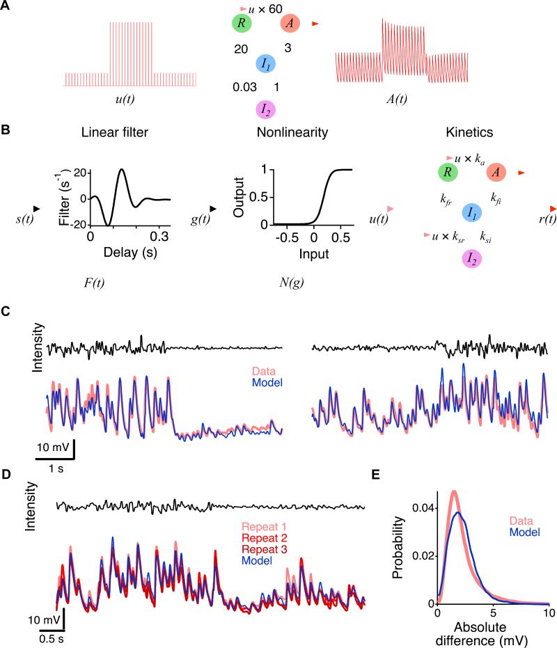
Figure 2. The Linear Nonlinear Kinetic (LNK) model.

A. A train of impulses that changed from low to high amplitude is shown as an input, u(t) presented to a first-order kinetic model with four states. Numbers indicate rate constants for transitions between the resting, R, active, A, and inactivated states, I₁ and I₂. The rate constant between resting and active states is modulated by u(t). The output is the occupancy of the active state, A(t). B. The LNK model. The input s(t) is convolved with a linear temporal filter, F_LNK(t) and then passed through a static nonlinearity, N_LNK(g) that does not change with contrast. The output of the nonlinearity u(t) controls two rate constants in the kinetics block, one that leads to the active state, and one that accelerates recovery from the inactivated state, I₂. Other rate constants are fixed, and the output of the model r′(t) is the active state. C. The membrane potential of an adapting amacrine cell compared to the LNK model output for a transition to low contrast (left) and to high contrast (right). D. The LNK model compared to the amacrine cell response for three repeats of an identical stimulus sequence. E. The distribution of the absolute difference in membrane potential between responses to an identical stimulus compared to the distribution of the difference between the model output and membrane potential responses. Results are combined for 6 cells with three repeated responses across the entire recording.