Comparison of Blood Flow Models and Acquisitions for Quantitative Myocardial Perfusion Estimation from Dynamic CT

Abstract

Myocardial blood flow (MBF) can be estimated from dynamic contrast enhanced (DCE) cardiac CT acquisitions leading to quantitative assessment of regional perfusion. The need for low radiation dose and the lack of consensus on MBF estimation methods motivates this study to refine the selection of acquisition protocols and models for CT-derived MBF.

Methods

DCE cardiac CT acquisitions were simulated for a range of flow states (MBF = 0.5, 1, 2, 3 ml/(min*g), cardiac output = 3, 5, 8 L/min). Patient kinetics were generated by a mathematical model of iodine exchange incorporating numerous physiologic features including heterogenenous microvascular flow, permeability and capillary contrast gradients. CT acquisitions were simulated for multiple realizations of realistic x-ray flux levels. CT acquisitions that reduce radiation exposure were implemented by varying both temporal sampling (1, 2, and 3 sec sampling intervals) and tube currents (140, 70, and 25 mAs). For all acquisitions, we compared three quantitative MBF estimation methods (two-compartment model, an axially-distributed model, and the adiabatic approximation to the tissue homogeneous model) and a qualitative slope-based method. In total, over 11,000 time attenuation curves were used to evaluate MBF estimation in multiple patient and imaging scenarios.

Results

After iodine-based beam hardening correction, the slope method consistently underestimated flow by on average 47.5% and the quantitative models provided estimates with less than 6.5% average bias and increasing variance with increasing dose reductions. The three quantitative models performed equally well, offering estimates with essentially identical root mean squared error (RMSE) for matched acquisitions.

Conclusions

MBF estimates using the qualitative slope method were inferior in terms of bias and RMSE compared to the quantitative methods. MBF estimate error was equal at matched dose reductions for all quantitative methods and range of techniques evaluated. This suggests that there is no particular advantage between quantitative estimation methods nor to performing dose reduction via tube current reduction compared to temporal sampling reduction. These data are important for optimizing implementation of cardiac dynamic CT in clinical practice and in prospective CT MBF trials.

Introduction

Quantitative assessment of myocardial blood flow (MBF) offers several clinical benefits over qualitative assessment of MBF including the potential to detect balanced ischemia and better grade the severity of ischemia, known to be strongly correlated to the occurrence of adverse cardiac events (Hachamovitch et al. 2002; Shaw et al. 2008). Positron emission tomography (PET, Kaufmann et al. 1999) and magnetic resonance imaging (MRI, Kroll et al. 1996) are two imaging modalities capable of quantitative MBF but are generally limited to larger academic centers with advanced imaging expertise. Quantitative assessment of MBF using dynamic cardiac CT has advantages over PET and MRI perfusion imaging in cost, availability, patient time in scanner, and spatial resolution.

Given these advantages, CT MBF imaging has been studied as a method to gain functional MBF information and to augment the anatomic information from coronary CT angiography (CTA). Two strategies to gain functional perfusion information are being developed, static and dynamic. In static CT perfusion, the relative enhancement of a myocardial region at a single time is used to indicate adequacy of perfusion. This approach has had some success (George et al. 2006; Rocha-Filho et al. 2010; Busch et al. 2011), however, it is only a relative measurement, requiring regions of normal perfusion in order to detect disease. Furthermore, the reliability of this method is challenged by the need to properly time the static acquisition post-injection of contrast. Dynamic CT perfusion, on the other hand, has the potential to detect balanced disease and measure perfusion in absolute units. The primary obstacle to general use of dynamic CT is the level of radiation imparted by repeated scanning; in current practice, these studies can result in an effective dose of 11 mSv to 54 mSv (Bamberg et al. 2012; So, Hsieh, Imai, et al. 2012; So, Hsieh, Li, et al. 2012). Clinical acceptance of dynamic CT requires lower dose acquisitions, and there is a lack of knowledge of the relative tradeoffs of myocardial blood flow estimation from dose-reduced studies.

A variety of models have been used to estimate perfusion information from the kinetics of a bolus of intravascular contrast agents. These methods range from qualitative approaches based on simplifying the kinetics to a few key metrics, such as rising slope and/or max level, to quantitative approaches based on optimizing models that incorporate spatially varying concentration gradients along the capillary bed. (Sourbron & Buckley 2012; Lee 2002). At present, there is currently no consensus on the optimal approach and vendors offer methods that provide disparate results (Goh et al. 2007). It is well appreciated that there are tradeoffs of sensitivity and noise with each method, dependent on the fidelity and sampling rate of input data. To address these competing problems, this work compares the performance of four common blood flow estimation methods on a wide range of realistic, CT-derived, time attenuation curves. Our goal was to determine optimal accuracy and precision for combinations of MBF estimation modeling and dynamic CT acquisition protocol for several viable dose reduction strategies including reduced x-ray flux (reduced tube current) and reduced temporal sampling.

Methods

Overview

In order to evaluate the accuracy and precision of various myocardial blood flow estimation methods, we started with a mathematical perfusion model based on physiologically guided blood-tissue exchange relationships. This gold-standard model included the effects of local myocardial flow heterogeneity, signal delay and dispersion in larger vessels, arterioles, and venules, and contrast agent escape into and recovery from capillary interstitial fluid. The predictions of this model drove the iodine dynamics in the ventricular cavities, aorta, and left ventricle myocardial tissue of a digital phantom under a variety of simulated cardiac outputs and myocardial perfusion levels. Simulated CT acquisitions of these dynamic digital phantoms yielded sinogram data that was reconstructed into many sets of temporally sequenced CT images. From each sequence of CT images, we extracted time attenuation curves (TACs) and estimated quantitative MBF with four different methods. An overview of the workflow is in Figure 1.

Figure 1. Process Overview.

A differential equation-based physiological model of cardiac blood flow dynamics is used to drive iodine contrast dynamics in a modified XCAT digital phantom. Physics-based simulated CT scans followed by image reconstruction with an iodine based beam hardening correction allows extraction of time attenuation curves (TACs) from regions of interest in myocardial tissue. Myocardial blood flow is estimated by fitting any of a variety of flow models to an extracted TAC. The example sequence shown in this figure is for a simulated patient with a cardiac output of 8 L/min, myocardial perfusion of 3 ml/(min*g tissue), who was scanned at 1 second/frame at 25 mAs and had four TACs examined from 3.25 × 3.25 mm² myocardial regions of interest (located at red dots in final CT image). The model fit example is for a 2-compartment model fitted to a TAC extracted for the apical myocardium.

Physiological Driving Model

The main features of the physiological driving model will be summarized here; more details are in the Appendix. The model was developed to represent iodine contrast transport in the blood from the right ventricle to the left atrium, left ventricle, myocardial tissue, and the descending aorta. Several publications have shown that transport through large cardiovascular vessels is well represented by a simple dispersive delay, characterized by a relative dispersion and a transit time (e.g. King et al. 1993). We use this representation to account for the changes in the iodine bolus profile between the right ventricle and left atrium, between the left atrium and left ventricle, and between the left ventricle and the descending aorta and myocardial region of interest.

Within myocardial tissue, local perfusion varies significantly even in normal healthy hearts (King et al. 1985; Bassingthwaighte et al. 1989), and this flow heterogeneity alters the tissue transport kinetics compared to monolithic flow. In our model, flow heterogeneity is represented by accounting for a multiplicity of tissue flows with various flow paths weighted according to an appropriate probability distribution (a slightly right-skewed lagged normal density curve). Each flow path has a representation of arteriolar, capillary, and venular transport, with perfusion level dependent exchange with interstitial fluid in the capillaries. The total iodine content for a piece of tissue is then the integral of the content along each path multiplied by the associated path weight. The model parameters were selected to be physiologically appropriate, drawn primarily from Bassingthwaighte (1987) and Vinnakota & Bassingthwaighte (2004).

This multi-stage model represents the key features of iodine dynamics in all the relevant regions of the heart. It is particularly relevant that we have captured the ventricular and aortic cavity iodine dynamics because these large pools of contrast agent can cause significant beam hardening artifacts in the relatively poorly enhanced myocardium, and these effects change significantly as the iodine bolus moves through the cardiovascular system. An important feature of any contrast enhanced CT-based myocardial perfusion assessment method will be its ability to deal appropriately with these artifacts.

Digital Phantom

The XCAT digital phantom (Segars et al. 2010) was modified so that the density associated with the right and left ventricular cavities, aorta, and left ventricle myocardial wall reflected the iodine dynamics predicted by the physiological driving model for a given cardiac output and myocardial blood flow level. To simulate a range of cardiac outputs and perfusion levels, we created 12 dynamic simulated patients from combinations of 3, 5, or 8 L/min cardiac output, and MBF levels of 0.5, 1, 2, or 3 ml/(min*g tissue). Images were generated at end diastole with no cardiac motion to mimic prospective cardiac gated acquisitions.

Simulated CT Scans

The CT acquisition simulation included the following components: 1) polychromatic fan-beam forward projection with a representative 120kVp spectrum, 2) quantum noise (compound Poisson distributed) with energy-weighting of Poisson variates corresponding to 1 keV energy bins, 3) and electronic noise (Gaussian distributed). The CT simulation followed conventional approaches such as those described in La Rivière et al. (2006). We simulated CT scanning of our 12 virtual patients over a period of 30 seconds, with scans every 1, 2, or 3 seconds, and with simulated tube currents of 140, 70, or 25 mAs. To ensure that the results we obtained were not dependent on a particular noise realization or the exact time window of the first scan, we began each set of scans at five different times spread equally over the temporal scanning window, and repeated each set of scans five times. Later analysis revealed that changes in starting time had no effect on flow estimation, so that the real effect was similar to having 25 different noise realizations for each scan of each patient with each tube current. In total, the parameters described led to 27,000 (=12 patients*30 scans*3 tube currents*5 noise realizations*5 scan start times) simulated sinograms. In addition, we were interested in examining the relative contributions of beam hardening artifacts and quantum and electronic noise to errors in flow estimation. In order to assess this we also ran simulated CT scans with noise turned off (conceptually equivalent to infinite tube current), since such scans will have beam hardening effects but no effects from noise. This leads to 1800 (=12 patients*30 scans*5 scan start times) noise-free simulated sinograms. For the purpose of comparison of CT techniques, the effective dose from these exams was estimated with the ImPACT CT Dosimetry Calculator (http://www.impactscan.org/ctdosimetry.htm).

Reconstruction and Iodine Beam Hardening Correction

From the 28,800 sinograms, CT images were reconstructed. It has previously been shown that beam hardening correction accounting for variations in iodine content is critical for dynamic cardiac CT (So et al. 2009). These images were iteratively improved with an image-based beam hardening correction algorithm (Stenner et al. 2010). This algorithm accounts for locations of soft tissue, bone, and iodinated contrast in the images, using temporal variation information to distinguish between bone and iodine. Applying this algorithm significantly reduces, but does not eliminate beam hardening artifacts in our images to reproduce the current best-practice application of clinical dynamic contrast enhanced CT.

TAC Extraction

In order to assess MBF estimation methods’ effectiveness in different areas of the myocardium, we examined four 5 pixel × 5 pixel (~11 mm²) regions of interest (ROIs) located in the basal, lateral, apical, and septal areas of the left ventricle myocardial wall (location presented on CT image of Figure 1). The mean CT number for each ROI in each image provides a datum along a time attenuation curve (TAC). This leads to a total of 3,840 (=12 patients*3 tube currents*(5 noise realizations+1 noisefree)*5 scan start times*4 ROIs) independent TACs where scans were performed once per second, 3,840 more by subsampling those to scans every two seconds, and 3,840 more by subsampling to scans every 3 seconds, for a total of 11,520 myocardial TACs for analysis. Along with each myocardial TAC, there is a 20 mm × 20 mm left ventricular cavity TAC, serving as the associated input function. These TACs include the attenuation due to blood, soft tissue, and contrast agent, so before the iodine enhancement can be determined, the non-contrast background signal needs to be removed. The earliest data point occurs before the arrival of contrast and its value is subtracted from the remaining curve to leave only the attenuation change due to iodine.

Flow Estimation Models

From the iodine-only TACs for the left ventricle cavity and a myocardial ROI, we evaluate four of the many possible methods for extracting perfusion information.

Maximum Slope Model (“Slope”)

The first, which we will refer to as the “Slope” method, is derived from the simple assumption that the rate of arrival of contrast agent is proportional to the tissue perfusion level. That is

$$\frac{d{C}_{\mathit{ROI}}(t)}{dt}=F·C_{in}(t)·\rho$$

where C_ROI is the concentration of contrast agent in the ROI (measured in Hounsfield Units (HU)), F is the myocardial blood flow (in ml/(min*g tissue)), C_in is the arterial input function (in HU), and ρ is the tissue density (in g/ml). This formulation implicitly assumes that no contrast agent exits the ROI in the time frame of the analysis and that there is no delay between the measured input function and the tissue arrival. This latter assumption can be relaxed by considering only the maximum values of C_in and dC_ROI/dt, and assuming any time difference represents the delay between input and tissue.

$$\underset{t}{max}\left(\frac{d{C}_{\mathit{ROI}}(t)}{dt}\right)=F·\left(\underset{t}{max}(C_{in}(t))\right)·\rho$$

Rearranging suggests we can estimate the MBF as

$$F=\frac{\underset{t}{max}\left(\frac{d{C}_{\mathit{ROI}}(t)}{dt}\right)}{\underset{t}{max}(C_{in}(t))}·\frac{1}{\rho }$$

the ratio of the maximum instantaneous slope of the myocardial iodine enhancement curve to the maximum value of the input function, multiplied by the reciprocal of the tissue density. For noisy curves, the instantaneous slope is extremely noisy, so in practice, the average slope along the upslope portion of the myocardial TAC is typically used instead (e.g. George et al. 2007; Bastarrika et al. 2010; Christian et al. 2004). If any contrast agent is leaving the ROI during the upslope of the myocardial TAC, the assumptions of the Slope method are violated and MBF will be underestimated.

Two Compartment Model (“2-Comp”)

The second flow estimation model is a two-compartment model (“2-Comp”) with a vascular and extravascular component connected through a permeable barrier. In this model, some contrast agent escapes from the blood into the interstitial fluid of as the iodine bolus passes through the myocardium, and then is more gradually washed back into the vascular bed. Since the contrast agent remains extracellular in both plasma and tissue, the total observed contrast agent at a time t is then the sum of its content in the blood plasma and in the interstitial fluid

$$C_{\mathit{ROI}}=(C_p{V}_p+C_{\mathit{isf}}{V}_{\mathit{isf}})·\rho$$

where C_p and C_isf are the plasma and interstitial fluid concentrations of contrast agent (in HU), and V_p and V_isf are the plasma and interstitial volumes (in ml/g tissue). The plasma and interstitial compartments are treated as well-mixed and contrast exchange between the two compartments is governed by the concentration difference between them and the capillary permeability-surface area product (PS).

$$\begin{array}{c}{V}_p\frac{d{C}_p}{dt}=F_p·\left(C_{{in}_p}-C_p\right)-PS·(C_p-C_{\mathit{isf}})\\ V_{\mathit{isf}}\frac{d{C}_{\mathit{isf}}}{dt}=PS·(C_p-C_{\mathit{isf}})\end{array}$$

where F_p is the plasma perfusion rate (in ml/(min*g)) and C_inp is the arterial input function for plasma arriving in the ROI, which is related to the measured arterial input function C_in by a delay (t_delay) and through the bulk hematocrit (H_bulk)

$$C_{{in}_p}(t)=\frac{C_{in}(t-t_{\mathit{delay}})}{1-H_{\mathit{bulk}}}$$

The plasma flow F_p is related to the tissue perfusion through the tissue discharge hematocrit (H_tD)

$$F=\frac{F_p}{1-H_{tD}}$$

Hematocrit can vary within local regions throughout the vasculature due to plasma skimming at vessel branches (where branching daughter vessels can receive a lower fraction of red blood cells due to their relative exclusion from the vessel wall) and the Fahraeus effect (a hydrodynamic effect in small vessels causing red blood cells to travel faster than the average plasma speed, leading to a lower dynamic hematocrit). For more discussion of the effects of hematocrit and a definition of the relationships between the bulk, tissue dynamic, and tissue discharge hematocrits, see the Appendix.

Two compartment models of this kind have been used to interpret data from dynamic CT (Brix et al. 1999; Cheong et al. 2004), MRI (Sourbron et al. 2009; Larsson et al. 2009; Brix et al. 2004), and PET (Larson et al. 1987).

Axially Distributed Model (“Distr”)

Instead of regarding the plasma and interstitial fluid compartments as well-mixed, the axially distributed model treats each as having spatial variation along one axis (Figure 3). This is a much more realistic representation of a capillary, which, due to being 100 times longer than its width, can support concentration gradients along its long axis while being considered well mixed across the short axis. The equations for this model are similar to the two compartment model except that instead of simply tracking the concentration for the complete compartment with time, contrast agent concentration is a function of time and axial position.

Figure 3. Flow estimation models.

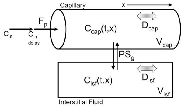
The model-based estimation methods can all be viewed as variants of an axially distributed tissue exchange model. First, a contrast agent input function (C_in) measured in the left ventricle travels to the capillary entrance, arriving some time (t_delay) after measurement. Once in the capillary three processes act on contrast agent, convection along the capillary length (flow, F_p), permeation of endothelial clefts into the surrounding interstitial fluid (governed by the permeability surface area product PS_g), and axial diffusion (diffusion coefficient D_cap). In the interstitial fluid there is no convection, only permeation and diffusion (D_isf). The full axially distributed model (“Distr”) allows contrast concentration gradients in both the capillary and interstitial fluid. The two compartment model (“2-Comp”) assumes complete mixing within the capillary and within the interstitial fluid (equivalent to assuming D_cap and D_isf→∞). and the adiabatic approximation to the tissue homogeneous model (“Adia”), the capillary space remains axially resolved, the interstitial space is considered well-mixed (D_isf→∞), and the exchange through permeation is simplified and considered to happen all at the distal end of the capillary.

$$\frac{\partial C_p(x,t)}{\partial t}=-\frac{F_{p}L}{V_p}\frac{\partial C_p}{\partial x}+\frac{PS}{V_p}(C_{\mathit{isf}}-C_p)+D\frac{{\partial }^2{C}_p}{\partial x^2}$$

where L is the length of the capillary, D is the contrast diffusion coefficient, and x is the location along the spatial dimension. The first term of this partial differential equation describes the convective flow of contrast through a point, the second describes exchange with the interstitial fluid, and the third describes diffusion. The equation governing the interstitial fluid concentrations is similar, except that there is no convective flow in the interstitium:

$$\frac{\partial C_{\mathit{isf}}(x,t)}{\partial t}=\frac{PS}{V_{\mathit{isf}}}(C_p-C_{\mathit{isf}})+D\frac{{\partial }^2{C}_{\mathit{isf}}}{\partial x^2}$$

Boundary conditions connect the upstream end to the input function and ensure that only convective flow in the capillary carries contrast out of the region

$$\begin{array}{l}{C}_p(0,t)=C_{{in}_p}\frac{\partial C_{\mathit{isf}}(0,t)}{\partial x}=0\\ \frac{\partial C_p(L,t)}{\partial x}=0\frac{\partial C_{\mathit{isf}}(L,t)}{\partial x}=0\end{array}$$

Axially distributed models have been applied to dynamic CT and MRI (Koh et al. 2003), and in PET (Larson et al. 1987).

Adiabatic Approximation to the Tissue Homogeneous Model (“Adia”)

Between the level of detail of the distributed model and the two compartment model, the tissue homogeneous model (Johnson & Wilson 1966) assumes that the interstitial fluid compartment is well-mixed while the plasma compartment is spatially distributed along one axis. St. Lawrence and Lee (1998) developed an approximation to this model which has been more widely used than the basic tissue homogeneous model due to the availability of a closed form solution in the time domain. Under the adiabatic assumption, changes in the interstitial contrast concentration are considered slow relative to changes in the intravascular contrast concentration, and therefore these two time scales can be handled separately. Instead of allowing exchange with the interstitium along the entire capillary, the adiabatic approximation assumes that the extracellular concentration has not changed much during the intravascular transit time and considers only the aggregate effect of exchange when the venous end is reached. The plasma concentration equation therefore has only a flow term

$$\frac{\partial C_p(x,t)}{\partial t}=-\frac{F_{p}L}{V_p}\frac{\partial C_p}{\partial x}$$

and the interstitial fluid concentration change depends only on extraction fraction (E) and the concentration difference between the interstitial compartment and the venous end of the capillary

$$\frac{\partial C_{\mathit{isf}}(t)}{\partial t}=E{F}_p(C_p(L,t)-C_{\mathit{isf}}(t))$$

where the extraction fraction is as defined in Crone (1963)

$$E=1-e^{-PS/F_p}$$

Model Fitting Procedure

In order to estimate MBF using the Slope method, the calculation first requires the maximum value of the background subtracted left ventricle input TAC and the slope of the rising portion of the background subtracted myocardial TAC. The shape of a single-pass bolus in the vascular system is often well-represented by a gamma variate function (Mischi et al. 2008). To reduce the effect of noise and sparse temporal sampling in the input function, we locate the peak by fitting with a gamma variate function, and the peak value of the gamma variate is used rather than the raw maximum of the input data. For easy parameterization, we use the formulation by Madsen (1992).

$$\gamma (t)={\gamma }_{\mathit{max}}{\left(\frac{t}{t_{\mathit{peak}}}\right)}^{\alpha }{e}^{\alpha \left(1-\frac{t}{t_{\mathit{peak}}}\right)}$$

This equation is fit to the input TAC data from the initial time, through the peak, until the input function falls to 50% of the peak value. Beyond this point, contrast recirculation causes significant deviations from the shape of a gamma variate.

To determine the slope of the rising portion of the background subtracted myocardial TAC, a line is fit to the portion of the myocardial TAC between 4 seconds before the time of the input function maximum to 7 seconds after the input function maximum or until the maximum of the myocardial TAC, whichever occurs earlier. This time window was empirically determined to do a reasonable job of covering the upslope window. Figure 2 shows example noisy input and myocardial TACs, as well as the associated gamma variate and line fits.

Figure 2.

Slope method. The “Slope” method calculates MBF from the ratio of the slope of the rising portion of the myocardial TAC to the peak value of the input function. We obtain the peak value of the input function by fitting a gamma variate to it and using the peak of the fit. We obtain the myocardial TAC slope by fitting a line to points between 4 seconds before the input peak and the peak of the myocardial curve or to 7 seconds after the input peak, whichever is sooner. Data points are from a virtual patient with cardiac output 3 L/min, MBF 3 ml/(min*g), tube current 140 mAs, and scans every 2 seconds.

For the other three models (2-comp, Distr, and Adia), the flow estimation procedure involved optimizing three parameters to minimize the least squares difference between the model-predicted myocardial iodine content and the extracted myocardial TAC, while holding all other parameters fixed at values which provided good fits to the ground truth myocardial curves (generated by the physiological driving model and undeformed by simulated scanning) for all 12 virtual patients. The three parameters optimized on were the perfusion level (F), the time delay between the input function and arrival in ROI (t_delay), and the volume of the interstitial fluid compartment in the ROI (V_isf).

To carry out the optimization, the models were formulated in JSim (Bassingthwaighte et al. 2006), a comprehensive and open source modeling platform, and the simplex (Dantzig et al. 1955) or sensop (Chan et al. 1993) optimizers were selected. Optimizations were performed to minimize the least squares error between the model predicted myocardial TAC and each of the 11,520 simulated TACs for each of these models. JSim project files containing all model parameters, equations, and optimization settings in a user-runnable form for the physiological driving model and the 2-Comp, Adia, and Distr models are available as Supplemental materials.

Results

Effects of Perfusion Level, Cardiac Output, and Tube Current on Regional Myocardial TACs

Cardiac output varies depending on physiologic conditions and results in advancing the rise and fall of myocardial TACs in time, without significantly affecting peak iodine enhancement (e.g. Fig 4A). In order to detect differences in MBF via dynamic CT, tissues with different perfusion levels must have differing time attenuation curves. This condition is clearly satisfied in high tube current scans (e.g. Fig 4C) where increases in MBF steadily increase the peak tissue enhancement and advance the rising edge of the enhancement curve in time. This information is generally preserved, but is much less obvious with the higher noise levels associated with reducing the tube current (e.g. Fig 4D). The noise level in low simulated tube current (25 mAs) scans renders the TACs extracted under varying cardiac outputs essentially indistinguishable (e.g., Fig 4B).

Figure 4. Example myocardial time attenuation curves (TACs) for varying cardiac outputs, perfusion levels, and simulated tube currents.

Panels A and B: Example lateral wall TACs for varying cardiac outputs (3, 5, or 8 L/min) and higher tube current (140 mAs, panel A) or lower tube current (25 mAs, panel B), at a true MBF of 2.0 ml/(min*g). Panels C and D: Example lateral wall TACs for varying MBF (0.5, 1, 2, or 3 ml/(min*g)) and higher tube current (140 mAs, panel C) or lower tube current (25 mAs, panel D) at a cardiac output of 5 L/min.

Estimated vs. True Myocardial Blood Flow Across Estimation Methods

The 2-Comp, Distr, and Adia models all provide myocardial blood flow (MBF) estimates with little bias at all tube currents and increasing standard deviation with decreasing tube current (see Figure 5 and Table 1). The Slope method consistently underestimates the MBF under all conditions, with the severity of the underestimation increasing with increasing true MBF.

Figure 5. Estimated myocardial blood flow (MBF) vs. true MBF across estimation models and at a variety of tube currents.

Noisefree TACs contain beam hardening effects from the simulated CT scan, but no quantum or electronic noise (equivalent to infinite tube current). Other panels simulate tube currents of 140, 70, or 25 mAs as noted. Bars are mean ± standard deviation of MBF estimates (180 estimates/bar for noisefree, 900 estimates/bar for others), horizontal dashed lines indicate the true MBF. Data is combined across cardiac outputs, noise realizations (for non-noisefree cases), temporal sampling schemes, and myocardial regions.

Table 1.

MBF Estimation Bias and Radiation Dose

Tube Current	140 mAs			70 mAs			25 mAs
Frame Interval (sec)	1	2	3	1	2	3	1	2	3
DLP* (mGy-cm)	1590	795	530	795	397.5	265	300	150	100
Effective Dose (mSv)	39	19.5	13	19.5	9.75	6.5	6.9	3.45	2.3
MBF Estimation Bias, mean ± std dev (ml/(min* g))
Two Compartment	−0.10 ± 0.47	−0.05 ± 0.53	0.02 ± 0.58	−0.08 ± 0.53	−0.01 ± 0.63	0.06 ± 0.72	−0.04 ± 0.83	0.06 ± 0.90	0.11 ± 0.99
Distributed	−0.08 ± 0.46	−0.03 ± 0.55	0.04 ± 0.60	−0.06 ± 0.52	0.02 ± 0.64	0.11 ± 0.77	0.04 ± 0.80	0.19 ± 0.95	0.26 ± 1.01
Adiabatic	−0.09 ± 0.46	−0.05 ± 0.54	0.03 ± 0.60	−0.08 ± 0.51	−0.00 ± 0.63	0.09 ± 0.77	0.01 ± 0.78	0.15 ± 0.93	0.22 ± 1.00
Slope	−0.94 ± 0.77	−0.95 ± 0.78	−0.95 ± 0.80	−0.94 ± 0.78	−0.93 ± 0.79	−0.94 ± 0.82	−0.92 ± 0.83	−0.88 ± 0.88	−0.95 ± 0.92

^*DLP = Dose Length Product

Effect of CT Protocol on MBF Estimate Error

Figure 6 shows the combined root mean square error (RMSE) across all estimates for each CT acquisition protocol, defined as a combination of a tube current and a temporal sampling frequency. All estimation methods are insensitive to temporal subsampling in the noisefree case. When realistic noise is present, for the three quantitative models (2-comp, Distr, Adia), RMSE increases similarly with reductions in tube current and with temporal subsampling. Points with similar total effective dose to the patient produce similar RMS error whether the dose reduction occurs via tube current reduction or reduced temporal sampling. For example, the 140 mAs and 2 second sampling and the 70 mAs and 1 second sampling acquisitions would both impart the same radiation dose and have an RMSE of ~0.55 ml/(min*g).

Figure 6. MBF estimation error dependency on tube current reductions and temporal subsampling.

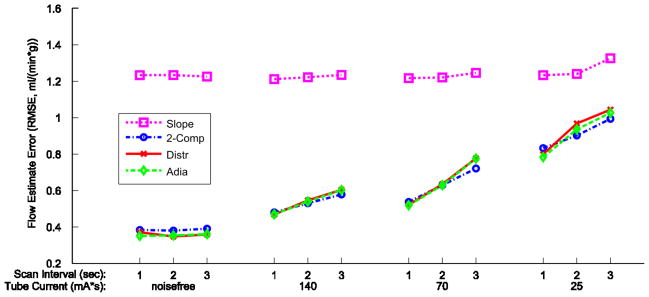
For each of the four MBF estimation methods, the root mean square error (RMSE) is calculated for all combinations of tube current and scan interval. Data points are the RMSE of all estimates combined across cardiac outputs, true MBF values, myocardial regions, and noise realizations, which is 240 estimates/point for the noisefree cases, and 1200 estimates/point for all others. Data for each estimation method/model has its own marker and line style as indicated in the legend.

Again, the Slope method behaves quite differently than the other methods, with a much higher overall RMS error of ~1.2 ml/(min*g), but is generally insensitive to increases in noise.

Tradeoff between MBF Estimation Error and Radiation Dose

Total patient radiation dose is the product of the radiation dose per scan and the number of scans. Figure 7 presents RMSE versus effective dose for all of the simulated acquisition schemes. As expected, reducing dose increases MBF estimation error but in a nonlinear fashion. Dose reductions from ~40 mSv to ~20 mSv, 20 to 10, and 10 to 5, increase error by 8%, 19%, and 35%, respectively. MBF estimation error is essentially independent of dose reduction strategy; i.e. reducing the tube current by half increases the estimation error by the same amount as reducing the number of scans by half without reducing tube current.

Figure 7. Tradeoff between MBF estimation error and radiation dose.

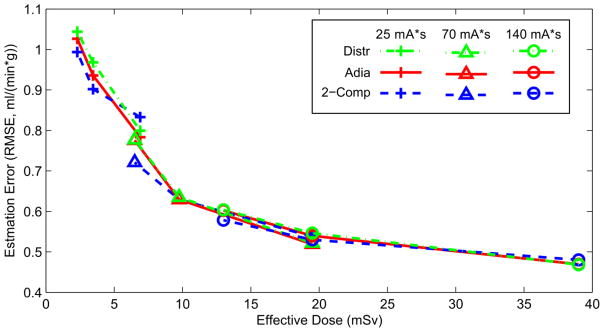
Both tube current reduction and temporal subsampling strategies are represented here. Each line style represents a different estimation model. A progression from circles (140 mAs) to triangles (70 mAs) to pluses (25 mAs) represents a reduction in tube current. Connected points have the same tube current time product and different temporal sampling, from 3 sec/frame on the left to 1 sec/frame on the right. RMS error is calculated across all TACs with the same dose, with data across cardiac outputs, true MBFs, and ROIs combined.

Estimation Method Reliability

TAC curve fitting failed to return a flow estimate due to numerical integrator errors in 769/46,080 cases (1.7%), so these realizations could not be included in further analysis. These errors primarily occurred in the Distr model at the lowest flow level. For the quantitative methods, the optimizer was limited to prevent MBF estimates below 0 ml/(min*g) or above 5 ml/(min*g); estimates at these limits indicate poor fitting and occurred in 393/46,080 (0.8%) of cases. For the qualitative Slope method, negative MBF estimates were returned when TAC deformations led to small negative myocardial slopes; this occurred in 238/46080 cases (0.5%). Negative and at-limit flow estimates were included in all analysis. All of these estimation failures represent a small fraction of total results and do not influence our reported conclusions.

Discussion

Cardiac CT imaging is primarily employed for assessing cardiac anatomy and coronary artery disease. Acquisition of a series of CT images as a contrast bolus progresses through the myocardium enables direct assessment of perfusion in order to determine the presence of myocardial ischemia. However, serial CT scans required for dynamic CT perfusion proportionately raise the radiation dose to the patient. Therefore, care must be taken to minimize the number of scans as well as the dose per scan, while retaining the clinically relevant information.

Prior studies have examined dynamic cardiac CT for MBF estimation. George et al. (2007) compared a two compartment model and two versions of an upslope method in an animal model of CT MBF and used microsphere-based MBF as the gold standard. They concluded that all three estimation methods correlate well with the microsphere MBF. However, the high correlations appear to be largely a result of the wide range of flows examined, and it is not suggested that any of these models provide quantitative estimates which are directly proportional to MBF. More recently, Bastarrika et al. (2010) compared dynamic cardiac CT assessment of MBF in humans to assessment by MRI. This group also used the upslope method, which was found to correlate well with the MRI upslope, reaching the same conclusions about perfusion defects with high sensitivity and specificity. These prior studies had a limited number of gold-standard measurements, evaluated only a single acquisition strategy, and generally tested a small set of potential models.

In contrast to prior studies, our dynamic cardiac CT simulation study evaluated the accuracy and precision of four myocardial blood flow estimation methods on twelve virtual patients under a range of CT image acquisition scenarios. The three quantitative model-based estimation methods all had very similar performance under all conditions tested and had essentially no systematic bias in quantitatively estimating MBF. The fourth MBF estimation method, the non-model based Slope method, consistently underestimates MBF in our simulations, a result that has been seen experimentally (e.g. George et al. 2007). This occurs because the underlying assumption of the Slope method is that no contrast agent has left the imaged tissue at the time of arrival of the input function peak. This assumption is simply not reasonable for myocardial tissue, especially in light of cardiac flow heterogeneity, which ensures very short transit times for some contrast agent.

While we have attempted to make our virtual patient contrast dynamics and simulated acquisitions very realistic, idealizations remain. The largest of these is that there is no cardiac motion within or between simulated scans. As gantry rotations speeds have increased and CT scan durations have fallen and shifted to being ECG-triggered, the ideal of frozen cardiac motion is more and more closely approached. Our iodine dynamics simulation does not account for all patient variability in iodine delivery and exchange. For example, we assume a fixed linear permeability relationship with flow and constant volumes of distribution (as discussed in appendix); two measures that probably vary with disease state. Moreover, each region in the virtual patients is assumed to have uniform density at each time point; this assumption includes the ventricular cavities where incomplete mixing can lead to non-uniformities.

Finally, we did not simulate several other physical effects of the CT acquisition, including photon scatter, detector efficiency non-uniformity, and within acquisition spectrum shifting.

The simulation system we have developed can be used to predict the estimation performance of any combination of estimation method and acquisition protocol. We have started with 4 methods, but others merit examination, including deconvolution methods (e.g. Lawrence & Lee 1998). Others who have attempted to validate dynamic CT perfusion estimation methods have suffered from difficulty in establishing an accepted and readily available gold standard for comparision. Radiolabeled or fluorescent microspheres, the most authoritative method, requires sacrifice of the animal (and obviously cannot be used in humans at all), which usually means a very small sample size and still entails ~13% measurement error (Alessio et al. 2013). The advantage of our simulation study was the ability to conduct thousands of experiments at low cost and with known absolute MBF levels and controlled conditions. However, this does not replicate the inconsistencies within a living being and future work to validate these results in clinical studies is critically important.

We find that equal reductions in radiation dose result in equal increases in RMSE estimation error, regardless of whether we achieve the dose reduction via reductions in tube current (noisier points) or reductions in temporal sampling (fewer points). This means that patient radiation dose reductions obtained through either tube current reduction and/or fewer CT scans could optimized for individual patients. For example, obese patients, where noise is expected to be high regardless of CT settings, may need more CT samples to maintain diagnostic MBF performance. Likewise, temporal sampling of the end diastole or systole phase can be dependent on the scanner capabilities and patient heart rate. Our results suggest that 1–3 second sampling are all equally effective for MBF estimation (assuming tube current is adjusting accordingly). Furthermore, while it is well appreciated that quantum noise (variance of pixel values) is, to first order, linear with tube current. Our results confirm that MBF estimation error is not linear with radiation dose. This knowledge, as presented in figure 7, could be used to guide acquisition techniques to achieve appropriate MBF estimates. For example, given an error tolerance, one could select the appropriate acquisition technique and blood flow model. Considering that dynamic CT can be a high dose procedure, having an acquisition technique tailored to minimize radiation dose is essential to perform these exams with as low as reasonably achievable (ALARA) levels. It should be stressed that we evaluated performance with a range clinically realistic CT settings but assume that this relationship will break down if tube current is reduced to the point of significant photon starvation and/or if temporal sampling becomes overly sparse.

Conclusion

Our ultimate goal is to provide dynamic cardiac CT recommendations for the optimal perfusion assessment method, including choice of CT acquisition scheme and estimation model. Our simulation study demonstrates that the Slope method is suboptimal for quantifying MBF. In addition, the three quantitative estimation methods we tested have essentially no MBF estimation bias, although the potential for substantial variance. RMSE of flow estimates rises exponentially as dose decreases. As a frame of reference, a 10 mSv dose entails a ~0.6 ml/(min*g) error and a 5 mSv dose entails a 35% increase to ~0.85 ml/(min*g) error. Between these three methods, we find no significant distinctions in the performances under a wide variety of conditions, and our error versus dose results suggest that there is no particular advantage to choosing dose reductions via tube current reduction or reduction in number of images within the limits tested. In clinical practice, however, individual frames may suffer from acquisition artifacts (for example, from inter- and intra-frame motion); this reality suggests that acquiring more temporal samples, each with lower dose, may be practically more advantageous than acquiring fewer temporal samples at a higher dose.

Appendix: Details of Physiological Driving Model

The physiological driving model is intended to represent the complexity of iodinated contrast bolus dynamics as it passes through the chambers of the heart, the large vessels, small arterioles, myocardial capillaries and interstitial fluid, and exits through venules (Figure A1). This representation includes details, such as regional flow heterogeneity, that affect iodine dynamics but are not typically included in MBF estimation models due to computation time or parameterization difficulties. The general approach was inspired by and the details are quite similar to the model presented in Kroll et al. (1996). Compared to the Kroll et al. model, we add postcapillary venules within the observation region, and also consider additional upstream steps to allow tracking of multiple ventricular iodine content curves important for accounting for beam hardening effects when scanned.

Figure A1. Model Overview.

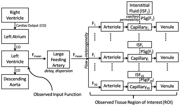
An input function observed in the left ventricle or aorta is carried by the mean blood flow (F_mean) through the large vessels into the microcirculation. Myocardial blood flow is significantly heterogeneous, and this is represented in the model by considering 20 different flow levels (F₁-F₂₀), where the flow levels are spaced to cover the range of relative flows. The parameters for all flow paths are identical except for the flow level and the capillary permeability (PSg_i), which is a linear function of the flow level. The iodine content for a tissue region of interest is considered to be the weighted sum of the contents of all the flow paths, where the weights are determined by the fraction of blood traveling at that flow level.

Large Vessels, Arterioles, and Venules

Contrast dynamics in all large vessels, arterioles, and venules (but not capillaries) uses a partial differential equation based vascular operator, representative of dispersive delay in a pipe. The outflowing contrast concentration (C_out,pipe(t)) is determined by the input (C_in,pipe(t)), mean transit time (t̄), and relative dispersion (RD). The governing equation is

$$\frac{\partial C_{\mathit{pipe}}(t,x)}{\partial t}=-\frac{1}{t}\frac{\partial C_{\mathit{pipe}}(t,x)}{\partial t}+\frac{1}{\overline{t}P}\frac{{\partial }^2{C}_{\mathit{pipe}}(t,x)}{\partial x^2}$$

with initial conditions uniformly zero and boundary conditions

$$\begin{array}{c}{\frac{\partial C_{\mathit{pipe}}}{\partial x}|}_{x=1}=0\\ \frac{1}{\overline{t}P}{\frac{\partial C_{\mathit{pipe}}}{\partial x}|}_{x=1}-\frac{1}{\overline{t}}\left(C_{\mathit{pipe}}{\mid }_{x=0}-C_{in,\mathit{pipe}}\right)=0\end{array}$$

where C_pipe(t,x) is the concentration profile in the pipe, t is time, x is the fractional progress through the pipe (i.e. x = 0 is the entrance and x = 1 is the outlet), and P is the Peclet number for the system (the dimensionless ratio between advective and diffusive velocities). The Peclet number fixes the degree of dispersion induced by passing through the system, and was set from the relative dispersion via the following empirical relationship

$$P=\frac{2}{{RD}^2}-2$$

This relationship is exact in the limit as P → 0 and P → ∞, and has a maximum error of ~5%. An approach used previously in similar models, the vascular operator of King et al. (1993) could not be used for our purposes because it can represent only a maximum relative dispersion of 0.48, whereas our method can represent any relative dispersion between 0 and 1.

The outflowing concentration from one pipe

$$C_{\mathit{out},\mathit{pipe}}(t)=C_{\mathit{pipe}}(t,x){\mid }_{x=1}$$

becomes the input concentration for the next segment.

For the large feeding artery, the flow is the mean flow to the ROI; within the ROI, twenty different flow levels are represented to capture the significant heterogeneity of flow levels even within the normal myocardium (King et al. 1985). The twenty flow levels are chosen to cover a range of relative flows from 0.05 to 3 times the mean flow and are weighted with a lagged normal density curve with mean of 1, relative dispersion 0.35, and skewness 1.3, a curve shown to approximate the probability density function of myocardial relative flows in baboon (King et al. 1985), rabbit (Gonzales & Bassingthwaighte 1990), and dog (Yipintsoi et al. 1973). Specifically, the range of relative flows is divided into twenty bins where the bin boundaries are equally logarithmically spaced. The flow level associated with each bin is the bin center, and the weight associated with each bin is the area under the curve within that bin.

For the large vessel operator between the left ventricle and the myocardial tissue of interest, a typical arterial relative dispersion of 0.18 was used, whereas the increased dispersiveness of smaller vessels were represented in the choice of 0.48 for small arterioles and venules within the region of interest.

Capillaries and Interstitial Fluid

At the capillary level, molecules of contrast agent can escape outward through endothelial clefts into the surrounding interstitial fluid, or be carried along with the plasma flow out into the draining venule. For each flow level, the input into each parallel capillary network is the outflow from the arteriole. Each set of parallel capillaries with identical flow is represented by a pair of equations (all symbols defined in Table A1):

$$\begin{array}{c}\frac{\partial C_{\mathit{cap}(i)}(t,x)}{\partial t}=-\frac{F_{p(i)}L}{V_{\mathit{cap}}}\left(\frac{\partial C_{\mathit{cap}(i)}(t,x)}{\partial x}\right)-\frac{{PS}_{g(i)}}{V_{\mathit{cap}}}(C_{\mathit{cap}(i)}(t,x)-C_{\mathit{isf}(i)}(t,x))+D\frac{{\partial }^2{C}_{\mathit{cap}(i)}(t,x)}{\partial x^2}\\ \frac{\partial C_{\mathit{isf}(i)}(t,x)}{\partial t}=\frac{{PS}_{g(i)}}{V_{\mathit{isf}}}(C_{\mathit{cap}(i)}(t,x)-C_{\mathit{isf}(i)}(t,x))+D\frac{{\partial }^2{C}_{\mathit{isf}(i)}(t,x)}{\partial x^2}\end{array}$$

with reflecting boundary conditions at the downstream ends of the interstitial fluid and capillary, as well as the upstream end of the interstitial fluid

$${\frac{\partial C_{\mathit{isf}(i)}}{\partial x}|}_{x=L}={\frac{\partial C_{\mathit{cap}(i)}}{\partial x}|}_{x=L}={\frac{\partial C_{\mathit{isf}(i)}}{\partial x}|}_{x=0}=0$$

The boundary condition at the upstream end of the capillary is more complicated.

$$D\frac{\partial C_{\mathit{cap}(i)}{\mid }_{x=0}}{\partial x}=\frac{F_{p(i)}L}{V_{\mathit{cap}}}(C_{\mathit{cap}(i)}-C_{\mathit{cap}(i)\_in})$$

This is a Robìn boundary condition to ensure that no material is lost upstream to diffusion. Together, the boundary conditions ensure that convection in the plasma is the only path for contrast agent to enter or leave the region of interest.

When attempting to estimate MBF from time attenuation curves, the effects of MBF and capillary permeability are intertwined (Jackson 2004); to unambiguously identify MBF, we must make an assumption regarding the extraction efficiency, which is governed by the permeability surface area product. The permeability surface area product (PS_g) has been shown to vary with the flow level (Cousineau et al. 1983; Cousineau et al. 1994; Caldwell et al. 1994), and a linear relationship fits the data adequately in all these cases.

$${PS}_g(F_{p(i)})={PS}_{g\_\mathit{Slope}}\left(\frac{F_{p(i)}}{1-{\mathit{Hct}}_{tD}}\right)={PS}_{g\_\mathit{Intercept}}$$

We set the slope and intercept parameters for this relationship by simultaneously optimizing them to fit several porcine myocardial TACs with differing MBF values (as measured by fluorescent microspheres; unpublished data shared by So and Lee, Robarts Research Institute).

Table A1.

Parameters

Parameter	Value	Definition	Reference
Fp(i)	(varies) ml/(min*g tissue)	Plasma flow at the ith flow level	-
Vcap	0.05 ml/g tissue	Capillary plasma volume	(Bassingthwaighte 1987)
L	0.1 cm	Capillary length	(Bassingthwaighte 1987)
D	10−6 cm2/sec	Axial diffusion coefficient for contrast agent	Estimated
Visf	0.16 ml/g tissue	Interstitial fluid volume	(Vinnakota & Bassingthwaighte 2004)
Vart	0.012 ml/g tissue	Arteriolar blood volume	Estimated1
Vven	0.018 ml/g tissue	Venular blood volume	Estimated1
VFA	0.016 ml/g tissue	Feeding artery blood volume	Estimated1
Hctbulk	0.45	Bulk hematocrit	Typical value
HcttD	0.45	Tissue “discharge” hematocrit	Based on (Crystal & Salem 1989; Pries et al. 1990)
HcttT	0.3825	Tissue “tube” hematocrit	Based on (Crystal & Salem 1989; Pries et al. 1990)
PSg_Slope	0.3853	Slope of PSg vs F line	(Cousineau et al. 1983; Caldwell et al. 1994)1,2
PSg_Intercept	0.3 ml/(min*g tissue)	Intercept of PSg vs F line	(Cousineau et al. 1983; Caldwell et al. 1994)1,2

¹Value estimated based on fitting to porcine dynamic cardiac CT TACs (Lee and So, personal communication);

²Linearity of relationship based on references

Table A2.

Variables

Variable	Definition
Ccap(i) (t,x)	Iodinated contrast concentration in the capillary with the ith flow level (HU)
Cisf(i) (t,x)	Concentration of contrast in interstitial fluid of capillary with ith flow level (HU)
Ccap(i)in (t)	Concentration of contrast entering capillary with ith flow level (HU)
PSg(i) (F)	Permeability surface area product for contrast agent passage through endothelial clefts
CFA (t)	Concentration of contrast in plasma of large feeding artery, not in ROI (HU)
Cart(i) (t)	Concentration of contrast in plasma of ROI arterioles (HU)
Cven(i) (t)	Concentration of contrast in plasma of ROI venules (HU)
CROI (t)	Total iodinated contrast concentration in the region of interest (HU)
CRV (t)	Concentration of contrast in plasma of right ventricle (HU)
CLV (t)	Concentration of contrast in plasma of left ventricle (HU)
CLA (t)	Concentration of contrast in plasma of left atrium (HU)
CDA (t)	Concentration of contrast in plasma of descending aorta (HU)

The total contrast agent in an ROI can be determined by summing the content of the arterioles, venules, capillaries, and interstitial fluid space contained in that ROI.

$$C_{\mathit{ROI}}(t)=\rho \sum _{i=1}^{20}{w}_i\left(V_{\mathit{art}}{C}_{\mathit{art}(i)}(t)+V_{\mathit{cap}}{\int }_0^L{C}_{\mathit{cap}(i)}(t,x)dx+V_{\mathit{isf}}{\int }_0^L{C}_{\mathit{isf}(i)}(t,x)dx+V_{\mathit{ven}}{C}_{\mathit{ven}(i)}(t)\right)$$

Right to Left Ventricle and Aorta

In order for our simulated scans to include realistic beam hardening effects, they need to include the large pools of contrast agent passing through the ventricles and aorta as the smaller enhancement builds in the myocardium. As noted above, mass transport from point to point in the cardiovascular system can generally be characterized by a dispersive delay, and we take this approach here as well. Using dynamic cardiac CT data from a healthy patient injected with a contrast bolus (Prof. Matthew Budoff, Los Angeles Biomedical Research Institute, personal communication), we first fit a gamma variate to the right ventricle TAC. Using this as the input function, we varied the mean transit time and relative dispersion to achieve an optimal fit to the next cavity in the sequence, the left atrium. The same procedure of adjusting mean transit time and relative dispersion allowed fitting the transition from left atrium to left ventricle. From the left ventricle to the descending aorta, the procedure is the same. This analysis provided us with estimates of the mean transit time and relative dispersion for a healthy human between the right ventricle and left atrium, left atrium and left ventricle, and left ventricle and descending aorta (Figure A2 and Table A3). Assuming a typical cardiac output of 5 L/min, we can assign effective volumes of blood between each of these points (since the mean transit time is the volume/flow). This results in an estimate of 500 ml blood between the right ventricle and left atrium, 100 ml effective blood volume between the left atrium and left ventricle, and 150 ml between the left ventricle and the descending aorta in the image plane (assuming the descending aorta receives 85% of the cardiac output). Once we have volume estimates, we can adjust the transit times to simulate the effects of different cardiac outputs.

Figure A2. Fitting Patient Iodinated Contrast Pools.

Symbols are data points drawn from a dynamic cardiac CT from a healthy patient. Dashed lines are model curves. Gamma variate parameters for right ventricle and transit time and relative dispersion parameters for all other transitions were iteratively adjusted until the shown fits were simultaneously achieved. Symbols: circles = right ventricle, triangles = left atrium, diamonds = left ventricle, squares = descending aorta.

Table A3.

Mean transit times and relative dispersions between large blood pools

Transition	Mean Transit Time (s)	Relative Dispersion
RV→LA	6.0	0.38
LA→LV	1.2	0.80
LV→DA	2.1	0.32

RV = right ventricle, LA = left atrium, LV = left ventricle, DA = descending aorta.

The input function we use for our simulations is the a gamma variate curve to the right ventricle TAC for the real patient data. This ensures that all our simulations have an identical injected mass of contrast agent and an realistic contrast bolus shape. Our parameterization follows the simplified form of Madsen (1992).

$$C_{RV}(t)=\{\begin{array}{c}0\text{if}t<t_{\mathit{delay}}\\ y_{\mathit{max}}{\left(\frac{t-t_{\mathit{delay}}}{t_{\mathit{peak}}}\right)}^{\alpha }exp\left(\alpha -\alpha \left(\frac{t-t_{\mathit{delay}}}{t_{\mathit{peak}}}\right)\right)\text{if}t\ge t_{\mathit{delay}}\end{array}$$

The best fit input curve for the right ventricle has y_max = 270 HU, t_peak=7 sec, and α =2.2. t_delay simply sets the time point at which the contrast concentration first rises from zero.

Hematocrit Considerations

Even within a single individual, hematocrit differs from organ to organ (Crystal & Salem 1989) and at different levels of the vasculature (Pries et al. 1990). This occurs chiefly because of two hydrodynamic effects, plasma skimming and the Fahraeus effect. In plasma skimming, a smaller side branch off of a larger vessel receives a lower proportion of red blood cells (RBCs) to plasma than the mother vessel because the flow streams nearest the vessel wall are relatively depleted of cells (because cell centers cannot be located at the wall due to the volume of the cell). This leads to a reduced hematocrit in the daughter branch and a slightly increased hematocrit in the mother branch. The Fahraeus effect is a dynamic reduction of hematocrit in small vessels where the average speed of red blood cells exceeds the average speed of the plasma (Albrecht et al. 1979). This effect is also due to the exclusion of RBC centers from a small zone near the wall of the vessel because, in small vessels, this means at the cells are always being pushed along by the fastest flow streams in the center of the vessel. The relative acceleration of the red blood cells leads to a decreased dynamic hematocrit compared to the hematocrit at the vessel entrance or exit. This is the case because the hematocrit at the inlet and outlet of the vessel represent the time-averaged arrival of RBCs and plasma, and if RBCs are traveling faster in the tube, then their volume-averaged hematocrit inside the tube must be less than in the reservoir they empty into.

We must take all this subtlety into account in our models because we need to track the concentration of contrast agent in the plasma, and our measurement tools give us only the iodine concentration in the blood (for ventricular measurements) or in whole tissue (for myocardial measurements), and the conversion factors we need involve the hematocrit in large blood pools (the bulk hematocrit, Hct_bulk), the volume-averaged hematocrit in myocardial tissue (the tissue “tube” hematocrit, Hct_tT), and the time-averaged hematocrit in myocardial tissue (the tissue “discharge” hematocrit, Hct_tD), all of which may be distinct from one another. The bulk hematocrit relates the blood pool contrast input function (C_{in_b}, which we measure directly) to the plasma input signal (C_in, which we need for the model).

$$C_{in}=C_{in\_b}·(1-Hc{t}_{\mathit{bulk}})$$

The tissue tube hematocrit relates the capillary plasma volume (V_cap) to the capillary blood volume (V_{cap_b}).

$$V_{\mathit{cap}}=V_{\mathit{cap}\_b}·(1-Hc{t}_{tT})$$

Finally, the tissue discharge hematocrit relates the blood flow (F_b) to the plasma flow (F_p).

$$F_p=F_b·(1-Hc{t}_{tD})$$

Clinical hematocrit values are drawn from relatively large pools of blood and reflect the bulk hematocrit. There have been limited studies on the possible values of the other hematocrits, but the available literature suggests that the dynamically reduced hematocrit in myocardial tissue is reduced by a factor of ~0.85 from the bulk hematocrit, and in other tissues the factor ranges from 0.6 (for duodenum) to 1.5 (for spleen) (Crystal & Salem 1989). This represents the net contribution of both hemodynamic effects. In vitro experiments with blood and glass tubes have demonstrated that the Fahraeus effect alone leads to a reduction factor between ~0.75 to 0.9 for tubes <100 μm (Pries et al. 1990). In reasonable agreement with these values, Gonzales & Bassingthwaighte (1990) found myocardial regional dynamic hematocrits to be 77% ± 9% of bulk hematocrit. For our model, we have chosen a ratio of myocardial tissue tube hematocrit to bulk hematocrit of 0.85, and a ratio of myocardial tissue discharge hematocrit to bulk hematocrit of 1.

Errors in the tissue discharge hematocrit, the least experimentally accessible hematocrit, translate directly to errors in blood flow estimation, independently of all other errors, as can be seen from the last of the hematocrit equations above. If we consider the possible range of the Fahraeus effect to be dynamic reductions to between 0.75–0.9, and take the combination of both effects to result in a reduction of 0.85 from the bulk hematocrit, then the range of possible values for myocardial discharge hematocrit/bulk hematocrit is from 0.94 to 1.13. For bulk hematocrits near 0.45, this translates to an error of ~−5% to ~+12% in MBF estimate (F_b), even if the plasma flow estimate (F_p) is perfectly accurate.

References

- Albrecht KH, et al. The Fahraeus Effect in Narrow Capillaries. Microvascular research. 1979;18:33–47. doi: 10.1016/0026-2862(79)90016-5. [DOI] [PubMed] [Google Scholar]
- Alessio AM, et al. Validation of an axially distributed model for quantification of myocardial blood flow. [Accessed November 5, 2013];Journal of nuclear cardiology. 2013 20(1):64–75. doi: 10.1007/s12350-012-9632-8. Available at: http://www.ncbi.nlm.nih.gov/pubmed/23081762. [DOI] [PMC free article] [PubMed] [Google Scholar]
- Bamberg F, et al. Accuracy of Dynamic Computed Tomography adenosine stress myocardial perfusion imaging in estimating myocardial blood flow at various degrees of coronary artery stenosis using a porcine animal model. [Accessed July 25, 2013];Investigative Radiology. 2012 47(1) doi: 10.1097/RLI.0b013e31823fd42b. Available at: http://journals.lww.com/investigativeradiology/Abstract/2012/01000/Accuracy_of_Dynamic_Computed_Tomography_Adenosine.12.aspx. [DOI] [PubMed] [Google Scholar]
- Bassingthwaighte JB, et al. GENTEX, a general multiscale model for in vivo tissue exchanges and intraorgan metabolism. [Accessed December 18, 2012];Philosophical transactions. Series A, Mathematical, physical, and engineering sciences. 2006 364(1843):1423–42. doi: 10.1098/rsta.2006.1779. Available at: http://www.ncbi.nlm.nih.gov/pubmed/16766353. [DOI] [PMC free article] [PubMed] [Google Scholar]
- Bassingthwaighte JB. The myocardial cell. Cardiology: Fundamentals and Practice. 1987:113–148. [Google Scholar]
- Bassingthwaighte JB, King RB, Roger SA. Fractal nature of regional myocardial blood flow heterogeneity. [Accessed August 22, 2012];Circulation Research. 1989 65(3):578–590. doi: 10.1161/01.res.65.3.578. Available at: http://circres.ahajournals.org/cgi/content/abstract/65/3/578. [DOI] [PMC free article] [PubMed] [Google Scholar]
- Bastarrika G, et al. Adenosine-stress dynamic myocardial CT perfusion imaging: initial clinical experience. [Accessed October 1, 2013];Investigative Radiology. 2010 45(6):306–13. doi: 10.1097/RLI.0b013e3181dfa2f2. Available at: http://scholar.google.com/scholar?hl=en&btnG=Search&q=intitle:Adenosine-Stress+Dynamic+Myocardial+CT+Perfusion+Imaging+Initial+Clinical+Experience#0. [DOI] [PubMed] [Google Scholar]
- Brix G, et al. Regional blood flow, capillary permeability, and compartmental volumes: measurement with dynamic CT--initial experience. Radiology. 1999;210(1):269–76. doi: 10.1148/radiology.210.1.r99ja46269. Available at: http://www.ncbi.nlm.nih.gov/pubmed/9885619. [DOI] [PubMed] [Google Scholar]
- Brix G, Kiessling F, Lucht R. Microcirculation and microvasculature in breast tumors: pharmacokinetic analysis of dynamic MR image series. [Accessed September 10, 2013];Magnetic …. 2004 doi: 10.1002/mrm.20161. Available at: http://onlinelibrary.wiley.com/doi/10.1002/mrm.20161/full. [DOI] [PubMed]
- Busch JL, et al. Myocardial hypo-enhancement on resting computed tomography angiography images accurately identifies myocardial hypoperfusion. [Accessed November 1, 2013];Journal of cardiovascular computed tomography. 2011 5(6):412–20. doi: 10.1016/j.jcct.2011.10.006. Available at: http://www.pubmedcentral.nih.gov/articlerender.fcgi?artid=3246505&tool=pmcentrez&rendertype=abstract. [DOI] [PMC free article] [PubMed] [Google Scholar]
- Caldwell JH, et al. Regional myocardial flow and capillary permeability-surface area products are nearly proportional. American journal of physiology. Heart and circulatory physiology. 1994;267:H654–H666. doi: 10.1152/ajpheart.1994.267.2.H654. [DOI] [PubMed] [Google Scholar]
- Chan I, Goldstein A, Bassingthwaighte J. SENSOP: a derivative-free solver for nonlinear least squares with sensitivity scaling. [Accessed October 22, 2013];Annals of biomedical engineering. 1993 21(6):621–631. doi: 10.1007/BF02368642. Available at: http://link.springer.com/article/10.1007/BF02368642. [DOI] [PMC free article] [PubMed] [Google Scholar]
- Cheong LHD, Lim CCT, Koh TS. Dynamic contrast-enhanced CT of intracranial meningioma: comparison of distributed and compartmental tracer kinetic models--initial results. [Accessed September 10, 2013];Radiology. 2004 232(3):921–30. doi: 10.1148/radiol.2323031198. Available at: http://radiology.rsna.org/content/232/3/921. [DOI] [PubMed] [Google Scholar]
- Christian T, et al. Absolute Myocardial Perfusion in Canines Measured by Using Dual-Bolus First-Pass MR Imaging. [Accessed October 3, 2013];Radiology. 2004 232:677–684. doi: 10.1148/radiol.2323030573. Available at: http://radiology.rsna.org/content/232/3/677.short. [DOI] [PubMed] [Google Scholar]
- Cousineau D, et al. Changes in cardiac transcapillary exchange with metabolic coronary vasodilation in the intact dog. [Accessed August 15, 2012];Circulation Research. 1983 53(6):719–730. doi: 10.1161/01.res.53.6.719. Available at: http://circres.ahajournals.org/cgi/doi/10.1161/01.RES.53.6.719. [DOI] [PubMed] [Google Scholar]
- Cousineau DF, et al. Microsphere and dilution measurements of flow and interstitial space in dog heart. [Accessed August 16, 2012];Journal of Applied Physiology. 1994 77:113–120. doi: 10.1152/jappl.1994.77.1.113. Available at: http://jap.physiology.org/content/77/1/113.short. [DOI] [PubMed] [Google Scholar]
- Crone C. The permeability of capillaries in various organs as determined by use of the “indicator diffusion” method. [Accessed September 10, 2013];Acta physiologica scandinavica. 1963 doi: 10.1111/j.1748-1716.1963.tb02652.x. Available at: http://onlinelibrary.wiley.com/doi/10.1111/j.1748-1716.1963.tb02652.x/abstract. [DOI] [PubMed]
- Crystal GJ, Salem MR. Blood volume and hematocrit in regional circulations during isovolemic hemodilution in dogs. Microvascular research. 1989;37(2):237–40. doi: 10.1016/0026-2862(89)90041-1. Available at: http://www.ncbi.nlm.nih.gov/pubmed/2725344. [DOI] [PubMed] [Google Scholar]
- Dantzig G, Orden A, Wolfe P. The generalized simplex method for minimizing a linear form under linear inequality restraints. Pacific Journal of Mathematics. 1955;5(2):183–195. Available at: http://msp.org/pjm/1955/5-2/p04.xhtml. [Google Scholar]
- George RT, et al. Multidetector computed tomography myocardial perfusion imaging during adenosine stress. [Accessed October 1, 2013];Journal of the American College of Cardiology. 2006 48(1):153–60. doi: 10.1016/j.jacc.2006.04.014. Available at: http://www.ncbi.nlm.nih.gov/pubmed/16814661. [DOI] [PubMed] [Google Scholar]
- George RT, et al. Quantification of myocardial perfusion using dynamic 64-detector computed tomography. Investigative radiology. 2007;42(12):815–22. doi: 10.1097/RLI.0b013e318124a884. Available at: http://www.ncbi.nlm.nih.gov/pubmed/18007153. [DOI] [PubMed] [Google Scholar]
- Goh V, Halligan S, Bartram CI. Quantitative Tumor Perfusion Assessment with Multidetector CT3: Are Measurements from Two Methods Commercial Software Packages Interchangeable? Radiology. 2007;242(3):777–782. doi: 10.1148/radiol.2423060279. [DOI] [PubMed] [Google Scholar]
- Gonzales F, Bassingthwaighte JB. Heterogeneities in regional volumes of distribution and flows in rabbit heart. [Accessed October 9, 2013];Am J Physiol Heart Circ Physiol. 1990 258(27):H1012–H1024. doi: 10.1152/ajpheart.1990.258.4.H1012. Available at: http://ajpheart.physiology.org/content/258/4/H1012.short. [DOI] [PMC free article] [PubMed] [Google Scholar]
- Hachamovitch R, Berman D, Kiat H. Value of Stress Myocardial Perfusion Single Photon Emission Computed Tomography in Patients With Normal Resting Electrocardiograms An Evaluation of. [Accessed July 23, 2013];Circulation. 2002 doi: 10.1161/hc0702.103973. Available at: http://circ.ahajournals.org/content/105/7/823.short. [DOI] [PubMed]
- Jackson A. Analysis of dynamic contrast enhanced MRI. [Accessed January 13, 2014];British Journal of Radiology. 2004 77(suppl_2):S154–S166. doi: 10.1259/bjr/16652509. Available at: http://bjr.birjournals.org/cgi/doi/10.1259/bjr/16652509. [DOI] [PubMed] [Google Scholar]
- Johnson J, Wilson T. A model for capillary exchange. [Accessed December 5, 2012];Am J Physiol -- Legacy Content. 1966 210(6):1299–1303. doi: 10.1152/ajplegacy.1966.210.6.1299. Available at: http://ajplegacy.physiology.org/content/210/6/1299.short. [DOI] [PubMed] [Google Scholar]
- Kaufmann Pa, et al. Assessment of the reproducibility of baseline and hyperemic myocardial blood flow measurements with 15O-labeled water and PET. Journal of nuclear medicine. 1999;40(11):1848–56. Available at: http://www.ncbi.nlm.nih.gov/pubmed/10565780. [PubMed] [Google Scholar]
- King RB, et al. A vascular transport operator. [Accessed August 24, 2012];Am J Physiol Heart Circ Physiol. 1993 265(6):H2196–2208. doi: 10.1152/ajpheart.1993.265.6.H2196. Available at: http://ajpheart.physiology.org/cgi/content/abstract/265/6/H2196. [DOI] [PMC free article] [PubMed] [Google Scholar]
- King RB, et al. Stability of heterogeneity of myocardial blood flow in normal awake baboons. [Accessed October 29, 2012];Circulation Research. 1985 57(2):285–295. doi: 10.1161/01.res.57.2.285. Available at: http://circres.ahajournals.org/cgi/doi/10.1161/01.RES.57.2.285. [DOI] [PMC free article] [PubMed] [Google Scholar]
- Koh TS, et al. A physiologic model of capillary-tissue exchange for dynamic contrast-enhanced imaging of tumor microcirculation. IEEE transactions on bio-medical engineering. 2003;50(2):159–67. doi: 10.1109/TBME.2002.807657. Available at: http://www.ncbi.nlm.nih.gov/pubmed/12665029. [DOI] [PubMed] [Google Scholar]
- Kroll K, et al. Modeling regional myocardial flows from residue functions of an intravascular indicator. [Accessed August 16, 2012];American Journal of Physiology-Heart and Circulatory Physiology. 1996 271:H1643–H1655. doi: 10.1152/ajpheart.1996.271.4.H1643. Available at: http://ajpheart.physiology.org/content/271/4/H1643.short. [DOI] [PMC free article] [PubMed] [Google Scholar]
- Larson K, Markham J, Raichle M. Tracer-kinetic models for measuring cerebral blood flow using externally detected radiotracers. [Accessed September 10, 2013];Journal of Cerebral Blood Flow & Metabolism. 1987 doi: 10.1038/jcbfm.1987.88. Available at: http://www.nature.com/jcbfm/journal/v7/n4/abs/jcbfm198788a.html. [DOI] [PubMed]
- Larsson HBW, et al. Measurement of brain perfusion, blood volume, and blood-brain barrier permeability, using dynamic contrast-enhanced T(1)-weighted MRI at 3 tesla. [Accessed August 20, 2013];Magnetic resonance in medicine. 2009 62(5):1270–81. doi: 10.1002/mrm.22136. Available at: http://www.ncbi.nlm.nih.gov/pubmed/19780145. [DOI] [PubMed] [Google Scholar]
- Lawrence K, Lee T. An adiabatic approximation to the tissue homogeneity model for water exchange in the brain: I. Theoretical derivation. [Accessed November 28, 2012];Journal of Cerebral Blood Flow & Metabolism. 1998 18:1365–1377. doi: 10.1097/00004647-199812000-00011. Available at: http://www.nature.com/jcbfm/journal/v18/n12/abs/9590489a.html. [DOI] [PubMed] [Google Scholar]
- Lawrence KS, Lee T. An adiabatic approximation to the tissue homogeneity model for water exchange in the brain: II. Experimental validation. [Accessed November 28, 2012];Journal of cerebral blood flow and …. 1998 18:1378–1385. doi: 10.1097/00004647-199812000-00012. Available at: http://ukpmc.ac.uk/abstract/MED/9850150. [DOI] [PubMed] [Google Scholar]
- Lee T-Y. Functional CT: physiological models. Trends in Biotechnology. 2002;20(8):S3–S10. Available at: http://linkinghub.elsevier.com/retrieve/pii/S0167779902020358. [Google Scholar]
- Madsen M. A simplified formulation of the gamma variate function. [Accessed February 20, 2013];Physics in Medicine and Biology. 1992 37(7):1597–1600. Available at: http://iopscience.iop.org/0031-9155/37/7/010. [Google Scholar]
- Mischi M, den Boer Ja, Korsten HHM. On the physical and stochastic representation of an indicator dilution curve as a gamma variate. [Accessed November 13, 2012];Physiological measurement. 2008 29(3):281–94. doi: 10.1088/0967-3334/29/3/001. Available at: http://www.ncbi.nlm.nih.gov/pubmed/18367805. [DOI] [PubMed] [Google Scholar]
- Pries aR, et al. Blood flow in microvascular networks. Experiments and simulation. [Accessed October 10, 2012];Circulation Research. 1990 67(4):826–834. doi: 10.1161/01.res.67.4.826. Available at: http://circres.ahajournals.org/cgi/doi/10.1161/01.RES.67.4.826. [DOI] [PubMed] [Google Scholar]
- La Rivière PJ, Bian J, Vargas Pa. Penalized-likelihood sinogram restoration for computed tomography. IEEE transactions on medical imaging. 2006;25(8):1022–36. doi: 10.1109/tmi.2006.875429. Available at: http://www.ncbi.nlm.nih.gov/pubmed/16894995. [DOI] [PubMed] [Google Scholar]
- Rocha-Filho J, et al. Incremental value of adenosine-induced stress myocardial perfusion imaging with dual-source CT at cardiac CT angiography. [Accessed October 17, 2013];Radiology. 2010 254(2) doi: 10.1148/radiol.09091014. Available at: http://radiology.rsna.org/content/254/2/410.short. [DOI] [PMC free article] [PubMed] [Google Scholar]
- Segars WP, et al. 4D XCAT phantom for multimodality imaging research. [Accessed October 31, 2013];Medical Physics. 2010 37(9):4902. doi: 10.1118/1.3480985. Available at: http://link.aip.org/link/MPHYA6/v37/i9/p4902/s1&Agg=doi. [DOI] [PMC free article] [PubMed] [Google Scholar]
- Shaw L, Berman D, Maron D. Optimal medical therapy with or without percutaneous coronary intervention to reduce ischemic burden results from the Clinical Outcomes Utilizing Revascularization. [Accessed July 23, 2013];Circulation. 2008 doi: 10.1161/CIRCULATIONAHA.107.743963. Available at: http://circ.ahajournals.org/content/117/10/1283.short. [DOI] [PubMed]
- So A, et al. Beam hardening correction in CT myocardial perfusion measurement. [Accessed October 1, 2013];Physics in medicine and biology. 2009 54(10):3031–50. doi: 10.1088/0031-9155/54/10/005. Available at: http://www.ncbi.nlm.nih.gov/pubmed/19398817. [DOI] [PubMed] [Google Scholar]
- So A, Hsieh J, Imai Y, et al. Prospectively ECG-triggered rapid kV-switching dual-energy CT for quantitative imaging of myocardial perfusion. [Accessed October 4, 2013];JACC Cardiovascular imaging. 2012 5(8):829–36. doi: 10.1016/j.jcmg.2011.12.026. Available at: http://www.ncbi.nlm.nih.gov/pubmed/22897997. [DOI] [PubMed] [Google Scholar]
- So A, Hsieh J, Li J-Y, et al. Quantitative myocardial perfusion measurement using CT perfusion: a validation study in a porcine model of reperfused acute myocardial infarction. [Accessed October 4, 2013];The international journal of cardiovascular imaging. 2012 28(5):1237–48. doi: 10.1007/s10554-011-9927-x. Available at: http://www.ncbi.nlm.nih.gov/pubmed/21800119. [DOI] [PubMed] [Google Scholar]
- Sourbron S, et al. Quantification of cerebral blood flow, cerebral blood volume, and blood-brain -barrier leakage with DCE-MRI. [Accessed September 10, 2013];Magnetic resonance in medicine. 2009 62:205–217. doi: 10.1002/mrm.22005. Available at: http://onlinelibrary.wiley.com/doi/10.1002/mrm.22005/full. [DOI] [PubMed] [Google Scholar]
- Sourbron SP, Buckley DL. Tracer kinetic modelling in MRI: estimating perfusion and capillary permeability. [Accessed July 13, 2012];Physics in medicine and biology. 2012 57(2):R1–33. doi: 10.1088/0031-9155/57/2/R1. Available at: http://www.ncbi.nlm.nih.gov/pubmed/22173205. [DOI] [PubMed] [Google Scholar]
- Stenner P, et al. Dynamic iterative beam hardening correction (DIBHC) in myocardial perfusion imaging using contrast-enhanced computed tomography. [Accessed September 6, 2013];Investigative radiology. 2010 45(6):314–23. doi: 10.1097/RLI.0b013e3181e0300f. Available at: http://www.ncbi.nlm.nih.gov/pubmed/20440212. [DOI] [PubMed] [Google Scholar]
- Vinnakota KC, Bassingthwaighte JB. Myocardial density and composition: a basis for calculating intracellular metabolite concentrations. [Accessed August 15, 2012];American journal of physiology. Heart and circulatory physiology. 2004 286(5):H1742–9. doi: 10.1152/ajpheart.00478.2003. Available at: http://www.ncbi.nlm.nih.gov/pubmed/14693681. [DOI] [PubMed] [Google Scholar]
- Yipintsoi T, et al. Regional Distribution of Diffusible Tracers and Carbonized Microspheres in the Left Ventricle of Isolated Dog Hearts. [Accessed October 4, 2012];Circulation Research. 1973 33(5):573–587. doi: 10.1161/01.res.33.5.573. Available at: http://circres.ahajournals.org/cgi/doi/10.1161/01.RES.33.5.573. [DOI] [PMC free article] [PubMed] [Google Scholar]
Associated Data
This section collects any data citations, data availability statements, or supplementary materials included in this article.