Tertiary structure-based prediction of conformational B-cell epitopes through B factors

Abstract

Motivation: B-cell epitope is a small area on the surface of an antigen that binds to an antibody. Accurately locating epitopes is of critical importance for vaccine development. Compared with wet-lab methods, computational methods have strong potential for efficient and large-scale epitope prediction for antigen candidates at much lower cost. However, it is still not clear which features are good determinants for accurate epitope prediction, leading to the unsatisfactory performance of existing prediction methods.

Method and results: We propose a much more accurate B-cell epitope prediction method. Our method uses a new feature B factor (obtained from X-ray crystallography), combined with other basic physicochemical, statistical, evolutionary and structural features of each residue. These basic features are extended by a sequence window and a structure window. All these features are then learned by a two-stage random forest model to identify clusters of antigenic residues and to remove isolated outliers. Tested on a dataset of 55 epitopes from 45 tertiary structures, we prove that our method significantly outperforms all three existing structure-based epitope predictors. Following comprehensive analysis, it is found that features such as B factor, relative accessible surface area and protrusion index play an important role in characterizing B-cell epitopes. Our detailed case studies on an HIV antigen and an influenza antigen confirm that our second stage learning is effective for clustering true antigenic residues and for eliminating self-made prediction errors introduced by the first-stage learning.

Availability and implementation: Source codes are available on request.

Contact: jinyan.li@uts.edu.au

Supplementary information: Supplementary data are available at Bioinformatics online.

1 INTRODUCTION

B-cell epitope is the binding site of an antibody on an antigen. It can be recognized by a specific B lymphocyte to stimulate an immune response. If both the antigen and its binding antibody are known, the epitope site can be accurately determined by wet-lab experiments, such as by X-ray crystallography. However, it takes a great deal of time and labor to identify the epitope(s) of an unknown antigen and its specific antibody. Computational methods have strong potential for efficient and large-scale epitope prediction for many antigen candidates at much lower cost. Early computational prediction methods have focused on the identification of linear epitopes, which are simple forms of B-cell epitopes.

A linear epitope is composed of a single continuous sequence segment. The early prediction methods have assumed that there should be a good and simple correlation between certain propensities and linear epitope residues, and attempted to predict linear epitopes through one or two propensities. For example, hydrophilicity was used by Hopp and Woods (1981) and Parker et al. (1986), flexibility by Karplus and Schulz (1985), protrusion index (PI) by Thornton et al. (1986), antigenic propensity by Kolaskar and Tongaonkar (1990), amino acid pair by Chen et al. (2007) and β-turns by Pellequer et al. (1993). To enhance the robustness of the prediction, various ideas of sliding windows have been proposed (Chou and Fasman, 1974) and applied in linear epitope prediction (Hopp and Woods, 1981; Karplus and Schulz, 1985; Westhof, 1993). However, the sliding window approach is oversimplified and the prediction performance was not improved significantly (Chen et al., 2007). In 2005, Blythe and Flower derived 484 amino acid propensity scales from the AAIndex and found that even the best set of scales and parameters performed only marginally better than random methods. They recommended the use of more sophisticated methods for epitope prediction (Blythe and Flower, 2005). Other research works have tried to use machine learning methods such as Hidden Markov Model (Larsen et al., 2006), Recurrent Neural Network (Saha and Raghava, 2006) and Support Vector Machine (Chen et al., 2007) to improve performance for linear epitope prediction.

The other form of B-cell epitope is called conformational epitope. A conformational epitope consists of discontinuous stretches of residues that are tightly connected after folding in 3D space. As over 90% of epitopes are conformational (Andersen et al., 2006) and an increasing number of protein structures have recently become available, close attention has been shifted to the problem of conformational epitope prediction (Andersen et al., 2006; Kulkarni-Kale et al., 2005; Lo et al., 2013; Moreau et al., 2008; Ponomarenko et al., 2008; Sun et al., 2009; Sweredoski and Baldi, 2008; Zhao et al., 2012). DiscoTope (Andersen et al., 2006) is one of the first methods to study conformational epitopes based on structural data. It combines the structural proximity sum of sequentially smoothed log-odds ratios with contact numbers to derive a prediction score. Another novelty of the method is that it uses the concept of structural window to smooth the physicochemical propensities. A later method called ElliPro (Ponomarenko et al., 2008) takes advantage of the PI (Thornton et al., 1986) and makes use of a residue clustering algorithm to predict both linear and conformational B-cell epitopes for a protein sequence or protein structure. ElliPro does not have a training process, but the parameter thresholds must be set before implementation. The SEPPA method (Sun et al., 2009) introduces a novel concept of ‘unit patch of residue triangle’ to describe the local spatial context of the protein surface. It also incorporates clustering coefficients to describe the spatial compactness of surface residues for epitope prediction. A more recent work in this area is the antibody-specific B-cell epitope prediction (Zhao et al., 2011). This method can accurately predict the more useful antibody-specific epitopes rather than antigenic residues. But it requires more prior information, e.g. antibody structure or sequence information. It is not applicable to a new virus when its antibody is unknown. In spite of intensive research, the prediction performance by all of these methods still needs much improvement.

In this work, we propose a much more accurate epitope prediction method named CeePre (Conformational epitope prediction). Two new ideas are adopted by CeePre. First, CeePre uses a new feature B factor in the learning process, combined with many other physicochemical, statistical, evolutionary and structural features of the residues. These features are also extended by a sequence window and a structure window to derive composite features. B factor is an important parameter of protein X-ray crystallography. It measures the flexibility/rigidity of residues/atoms in a protein 3D structure. A higher B factor score implies more flexibility of the atom/residue. It has been found that low B factors are usually distributed at the core of unbound interfaces (Swapna et al., 2012). The second new idea is that CeePre is a two-stage model under the random forest learning process (Breiman, 2001). In the first stage, the original 304 features are used to predict the potential antigenic residues. In the second stage, the predicted class labels from the first stage are added to the feature space to cluster nearby antigenic residues to form epitopes and remove isolated antigenic or non-antigenic residue predictions. This idea is based on the hypothesis that the aggregated antigenic residues are more likely to constitute epitopes, while the isolated antigenic residues are probably wrongly predicted. This idea is effective to eliminate self-made prediction errors to obtain really meaningful final results.

CeePre is tested on a set of 55 epitopes from 45 tertiary antigen structures. The result shows that CeePre significantly outperforms all existing structure-based epitope predictors (DiscoTope, ElliPro and SEPPA). With a comprehensive analysis of the important features suggested by random forests in the epitope prediction, it is found that B factor, relative accessible surface area (RSA) and PI play an important role in improving prediction performance. Our analysis also confirms that whether a residue is involved in an epitope is affected by nearby residues both in sequence and in space, and thus it is a good idea to use both the sequence and structure window to construct the feature vector.

2 MATERIALS AND METHODS

2.1 Datasets

The structure data in this work consists of two types: quaternary structures and tertiary structures. Quaternary structures are used to determine which residues are in an epitope, while tertiary structures are used to extract feature scores of candidate residues. The structure data are compiled via the steps presented below.

2.1.1 Quaternary structures and epitope residues

A dataset containing 107 non-redundant antigen–antibody complexes (Kringelum et al., 2013) is used. Some (e.g. T-cell antigens) are removed according to the following criteria.

• Only one symmetric unit is used within each complex. If a complex contains more than one symmetric unit, redundant units are removed, as carried out by Ponomarenko and Bourne (2007).

• Complexes 1NFD, 1XIW, 1YJD and 2ARJ are removed because their antibodies interact only with the T-cell chains and have no interaction with antigen chains. 1QFW is also removed because its antigen chains are from the gonadotropin alpha subset.

In total, 102 quaternary structures are used to determine the B-cell epitopes. An epitope residue is an antigen residue such that there exists at least one heavy atom of this antigen residue that is within 4 Å distance from a heavy atom of a residue of the antibody (Ponomarenko et al., 2008).

2.1.2 Tertiary structures

Traditional structure-based epitope prediction methods typically use quaternary structure datasets (Andersen et al., 2006; Kringelum et al., 2013; Sun et al., 2009). From a practical perspective, the prediction should be conducted under the assumption that the corresponding antibodies are unknown. In other words, using tertiary structures rather than quaternary structures is more reasonable for the analysis and prediction of epitopes. Simply separating the antigens from the quaternary structures is not a good idea to get the tertiary structure data. This is because the antigen side in a quaternary structure contains the binding information (Supplementary Fig. S1); for example, residues bound by antibodies are less flexible and have smaller B factors in the quaternary structure. It is unfair to use the binding information to predict epitope sites in an unbound status. Therefore, to obtain the corresponding tertiary structures of the antigens from the quaternary structures is non-trivial.

We take an alignment approach to the construction of our tertiary structure dataset from the quaternary structure data. First, the antigens in the quaternary structures are aligned with every tertiary structure in Protein Data Bank (PDB). A tertiary structure is selected if the sequence similarity is >95% and the epitope residues can be completely aligned. By this step, 34 complexes are removed, as they cannot be aligned with any tertiary structure under the 95% sequence similarity condition. 1EGJ is also removed because it can only be aligned with 1C8P, which is determined by NMR (not X-ray). Twelve more complexes are removed because their epitopes cannot be completely mapped onto the corresponding tertiary structures.

After this filtering process, 55 quaternary structures are retained and their corresponding epitopes are mapped onto 45 tertiary structures. For some cases, two or more antigens from quaternary structures are mapped onto the same tertiary structures. Supplementary Table S1 shows the dataset details and the mapping between the quaternary structures and the tertiary structures. All the feature scores of the residues in this work are extracted from the tertiary structures rather than the quaternary structures.

2.1.3 Non-epitope residues

In general, except for epitope residues all other surface residues in a tertiary structure can be considered to be non-epitope residues. In particular, Rost and Sander (1994) have considered a residue to be a surface residue if its RSA is >15%, while the RSA threshold is set at 25% by Deng et al. (2009). The absolute value of the accessible surface area (ASA) has also been used to identify surface residues. Jordan (2010) has adopted a threshold of 5 Ų to define surface residues. Using a simple statistic on the RSA of epitope residues in our dataset, we find that >75% of epitope residues have an RSA >25.9%. Thus, we take the criterion RSA 25% (Deng et al., 2009) to define surface residues. As a result, there are 725 epitope residues and 6504 non-epitope residues in our datasets.

A key issue here is that the numbers of epitope residues and non-epitope residues are imbalanced. The epitope residues are just a little more than 10% of the non-epitope residues. If this imbalanced dataset is used in training, the classifier would tend to categorize every residue as non-epitope. Therefore, we sample non-epitope residues randomly to obtain the same number of non-epitope residues as that of the epitope residues to produce a balanced dataset. CeePre is trained on these balanced datasets and tested on both the balanced dataset and the imbalanced dataset.

2.2 Feature space of residues

2.2.1 Basic features including our newly proposed B factor

A variety of features have been studied by Chen et al. (2007); El-Manzalawy et al. (2008); Hopp and Woods (1981); Janin (1979); Karplus and Schulz (1985); Kolaskar and Tongaonkar (1990); Pellequer et al. (1993); Sollner et al. (2008); Thornton et al. (1986). In addition to our newly introduced B factor feature to characterize epitope residues, many of those traditionally used physicochemical features, statistical features, evolutionary features and structural features are also collected by this work (Table 1). In total, there are 38 features as our basic features (Supplementary Table S2), including 20 PSSM features and 8 secondary structure features. The B factor score of each residue is the average B factor of all of the atoms in this residue.

Table 1.

Features used in the our study and the methods for calculating their value scores

Catalogue	Feature	Calculation
Physicochemical	Hydrophilicity	Parker (Andersen  et al., 2006)
	Hydrophobicity	AA Index (Kawashima  et al., 2008)
	Flexibicity	AA Index (Kawashima  et al., 2008)
	Polarity	AA Index (Kawashima  et al., 2008)
	β-turns	AA Index (Kawashima  et al., 2008)
	B factor	PDB file
Statistical	Log-odds ratio	DiscoTope (Andersen  et al., 2006)
Evolutionary	PSSM	PSI-Blast
Structural	PI	PSAIA (Mihel  et al., 2008)
	ASA	NACCESS
	RSA	NACCESS
	Secondary structure	DSSP

2.2.2 Window-based features: extended composite features

The location of epitope residues can be influenced by their nearby residues in sequence and spatially. We introduce two windows to capture this influence: a sequence window and a structure window. Features whose value scores are calculated according to the residues within a window are called window-based features.

• A total of 38 smoothed features by a sequence window. The size of the sequence window is 7 (Andersen et al., 2006), i.e. the sequence window of a residue i covers residues i − 3, i − 2, i − 1, i, i + 1, i + 2, i + 3. We use the average value of each basic feature v over this window to obtain the smoothed value of v for residue i. It is named a smoothed feature v′. As there are 38 basic features, we can obtain an additional 38 smoothed features for each residue. Note that the window size is adjustable.

• A total of 228 new features by a structure window. A surface residue is inside a structure window of a target residue if the distance between any atom of the target residue and an atom of the surface residue is less than a threshold (window size: 10 Å, adjustable). We calculate the maximum, minimum and average of all of the residues in the structure window of each residue for every basic or sequence-window smoothed feature u. This process introduces 228 [(38 + 38) × 3] composite features, which are named structural maximum, minimum or average features of u. With this addition, we use a total of 304 (38 + 38 + 228) features to characterize every residue.

Figure 1 summarizes the process of constructing feature space from tertiary structures.

Fig. 1.

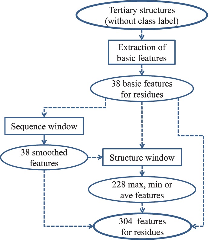
Construction of the feature space from tertiary structures

2.3 Prediction method

2.3.1 Two-stage learning

Our prediction method CeePre has two stages of learning:

• The first stage of learning is by the random forest model (Breiman, 2001) on a training dataset of residues described by our 304 features. The trained model is named CeePre1. CeePre1 can predict the class labels of the residues in a test dataset. It can also predict the class labels of the training residues. CeePre1 is depicted in Figure 2.

• The second stage of learning consists of four steps. Step 1: train a CeePre1 model on a training dataset described by the 304 features, and obtain the predicted class labels for the training data and the test data. The predicted class labels of the training data are given by an internal 10-fold cross-validation process over the training data itself. Step 2: expand the 304-feature vector by adding four features through a structure window and the predicted class labels of CeePre1. The four new features of the residues are (i) the predicted class label of CeePre1, (ii) the number of predicted epitope residues in the window, (iii) the number of predicted non-epitope residues in the window and (iv) the ratio of the predicted epitope residues over all the residues in the window. Step 3: train the random forest model on the enriched training dataset described by 308 features. The trained model is named CeePre2. Step 4: apply CeePre2 to predict the class labels of the residues in the test dataset described by the same 308 features and to get the test performance. Figure 3 illustrates the learning and test processes of CeePre2.

Fig. 2.

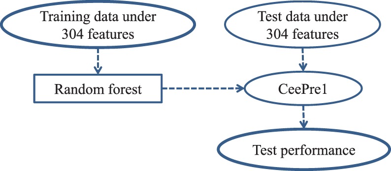
The learning and test of CeePre1

Fig. 3.

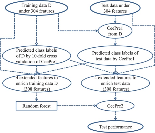
The learning and test of CeePre2

CeePre1 focuses on the accurate prediction of antigenic residues. On top of CeePre1, CeePre2 concentrates to cluster separate antigenic residues and to eliminate isolated false positives and false negatives. Generally, spatially aggregative antigenic residues more easily constitute epitopes. On the contrary, isolated antigenic residues are not likely to be a part of an epitope. Taking this principle, CeePre2 converts the prediction results of CeePre1 into the four features at the second stage to integrate separated antigenic residues into a cluster of epitope residues, enhancing the prediction performance for many cases.

2.3.2 Random forest

Random forest is used as our learning model. Random forest is an ensemble method proposed by Breiman (2001). It constructs multiple decision tree classifiers and obtains the final predictions by voting. It has many advantages (Han et al., 2006). Firstly, it is robust to errors and outliers and can avoid over-fitting. Secondly, its accuracy is comparable with other ensemble algorithms (e.g. AdaBoost), but it is much faster. Also, it gives an internal estimate of variable importance.

Many software packages contain the random forest algorithms. An implementation of random forest in R package by Liaw and Wiener (2002) is used here. There are two important parameters: the number of trees to grow and the number of features selected as candidates at each split. In the learning process, we build 100 trees and determine feature numbers by optimizing F-score.

2.4 Evaluation metrics

CeePre is evaluated under six metrics: accuracy, recall, specificity, precision, F-score and Matthews correlation coefficient (MCC). Recall, specificity and precision reflect the prediction tendencies of classifiers. Recall (sensitivity or TP recognition rate) and specificity (TN recognition rate) illustrate the percentage of correct predictions for positive and negative samples. A corresponding criterion is precision showing the percentage of correct positive-labeled samples. There is a trade-off between precision and recall. Recall favors positive-bias predictions, while precision favors negative predictions.

Accuracy (recognition rate) describes how well the classifier recognizes both positive samples and negative samples. It is effective only when the samples are evenly distributed. If positive and negative samples are imbalanced, classifiers apt to predict samples, as the majority class will achieve better accuracy. The F-score combines precision and recall and can be used to assess the performance of classifiers on both balanced datasets and imbalanced datasets. MCC is another metric that can be used to evaluate a classifier’s performance, especially on imbalanced datasets. It returns a value between −1 and +1: +1 stands for a perfect prediction, 0 for random prediction and −1 for totally reversed prediction.

3 RESULTS AND DISCUSSION

We first compare our CeePre model with three other structure-based epitope predictors (DiscoTope, ElliPro, SEPPA). The evaluation is based on both the balanced datasets and the whole imbalanced dataset. In this section, we also highlight several B factor-related features, which are important in epitope prediction.

3.1 Evaluation on the balanced datasets

A 10-fold cross validation procedure is conducted on our balanced datasets consisting of all the 725 epitope residues and 725 non-epitope residues obtained by sampling. The sampling is operated three times to obtain three different non-epitope residue datasets. The mean value and standard deviation of each metric over the three samplings are reported to eliminate the bias induced by sampling.

The performance of CeePre and those of the other three predictors are presented in Table 2. CeePre (CeePre1 and CeePre2) exhibits excellent performance on the balanced datasets, surpassing the other three predictors on all metrics. Specifically, the F-score of CeePre2 is 0.89, 0.31 higher than the best F-score (SEPPA) of the other predictors. The MCC of CeePre2 is 0.77, which is four times more than the best MCC of the other three predictors (0.19 by SEPPA). Accuracy is meaningful on the balanced datasets: the accuracy of CeePre2 is 0.88, 0.29 better than the best accuracy (SEPPA) of the other predictors. In summary, CeePre shows excellent performance on the balanced datasets.

Table 2.

Performance on the balanced datasets

Methods	F-score	Precision	Recall	MCC	Specificity	Accuracy
CeePre1	0.85 ± 0.013	0.85 ± 0.012	0.85 ± 0.016	0.71 ± 0.026	0.85 ± 0.012	0.85 ± 0.013
CeePre2	0.89 ± 0.006	0.85 ± 0.009	0.93 ± 0.003	0.77 ± 0.014	0.83 ± 0.011	0.88 ± 0.007
DiscoTope	0.33 ± 0.004	0.57 ± 0.022	0.23 ± 0.000	0.07 ± 0.020	0.83 ± 0.015	0.53 ± 0.008
ElliPro	0.61 ± 0.001	0.51 ± 0.001	0.76 ± 0.000	0.03 ± 0.004	0.27 ± 0.003	0.51 ± 0.002
SEPPA	0.58 ± 0.007	0.60 ± 0.016	0.56 ± 0.000	0.19 ± 0.025	0.63 ± 0.025	0.59 ± 0.012

Note: a ± b represents mean value a and standard deviation b.

We can also see that CeePre2 outperforms CeePre1 in terms of almost all metrics except for slight decrease in specificity. For example, the recall of CeePre2 is improved to 0.93 because more epitope residues are identified. The improvement is attributed to the idea that CeePre2 adds the prediction results of CeePre1 into the four new features expanded in the second learning stage. CeePre2 also removes some isolated epitope and non-epitope residue predictions and clusters nearby epitope residue and non-epitope residue predictions. This is reasonable because all residues in an epitope are typically spatially close to each other. On the other hand, one or two isolated residues should not become an epitope. The slight decrease in specificity probably implies the discovery of previously unknown epitopes in the tertiary structures, as the epitopes have not been fully annotated so far.

3.2 Evaluation on the whole dataset

In a real scenario, the number of epitope residues and non-epitope residues are not equal. To make the results more convincing in practice, we show a 10-fold cross validation result on the entire dataset, where the proportion of epitope residues and non-epitope residues is 1:9. For each fold, the training is on nine parts of the balanced dataset, and the test is on one part of the epitope residue data and all of the remaining non-epitope residues (not only the one part of the non-epitope residue data in the balanced dataset). The 10-fold cross validation process is repeated three times each with a different sampling of the non-epitope residues. The mean value and the standard deviation of each criterion are recorded in Table 3.

Table 3.

Performance on the whole dataset

Methods	F-score	Precision	Recall	MCC	Specificity	Accuracy
CeePre1	0.55 ± 0.019	0.41 ± 0.025	0.85 ± 0.016	0.53 ± 0.016	0.86 ± 0.016	0.86 ± 0.013
CeePre2	0.54 ± 0.006	0.38 ± 0.007	0.93 ± 0.003	0.53 ± 0.005	0.83 ± 0.006	0.84 ± 0.005
DiscoTope	0.16	0.13	0.23	0.04	0.82	0.76
ElliPro	0.18	0.10	0.76	0.02	0.27	0.32
SEPPA	0.23	0.14	0.56	0.11	0.62	0.62

Note: Sign a ± b represents mean value a and standard deviation b.

Again CeePre has far better performance than the other three predictors under all metrics. It achieves an F-score of 0.54, which is twice as much as the best F-score (SEPPA) of the other three predictors. Its MCC is ∼0.53, while the best MCC of the others is only 0.11. Compared with CeePre1, its recall improves significantly to 0.93, indicating that most of the epitope residues are identified. However, the precision and specificity of CeePre2 show a slight decrease, which is partly due to the incomplete determination of epitopes in PDB.

CeePre also has better recall, precision and specificity than the other three predictors. In terms of specificity, DiscoTope has a higher specificity (0.82) than ElliPro and SEPPA, which is slightly less than the specificity of CeePre2, but the recall of DiscoTope is only 0.23. This signifies that DiscoTope mistakes most of the epitope residues for non-epitope residues. In contrast, ElliPro prefers to recognize more residues as epitope residues, and thus shows a high recall value (0.76) and a low precision (0.1). Nevertheless, its recall is still much less than the recall of CeePre. This is probably because ElliPro only uses one feature (PI) in the prediction. SEPPA compromises epitope residue predictions and non-epitope residue predictions; thus, it has medium recall and specificity, but higher precision than the other two. However, the highest values of all three metrics of the other three predictors are lower than those obtained by our CeePre method.

3.3 Important features for prediction

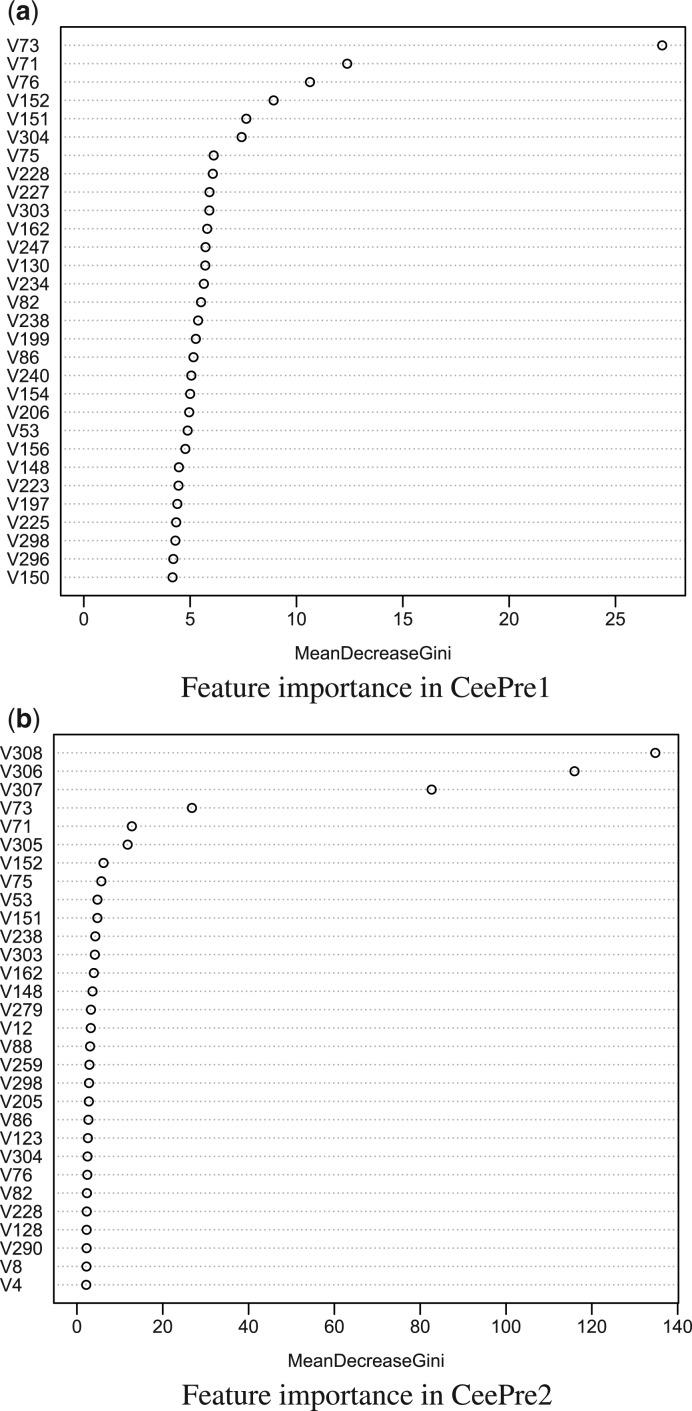
A variety of features, including physicochemical features, statistical features, evolutionary features and structural features, are used by CeePre. Not all of them play an equally important role in the prediction. Their contribution to the prediction performance varies. The most effective features should have both significant biological and computational importance. In this section, we report the most important features for epitope prediction. These features are ranked by the random forest model, as shown in Figure 4.

Fig. 4.

Ranking of top-30 important features in CeePre. (a) Shows the top-30 important features in the original 304 features. (b) Illustrates the top-30 important features of all the 308 features in CeePre2. In CeePre2, the four additional features are the prediction result of CeePre1 (V305), the number of predicted epitope residues in the structure window (V306), the number of predicted non-epitope residues in the structure window (V307) and the rate of predicted epitope residues in the structure window (V308)

Figure 4b shows that the four new features extracted from the prediction results of CeePre1 by a structure window do play a significant role in CeePre2, indicating a strong clustering effect. Other features, especially RSA (V73) and ASA (V71), are also top ranked in CeePre2. Figure 4a gives a more detailed description of the weighty features for characterizing epitope residues. This ranking procedure is repeated on three training samplings. Only those features that appear three times in the top-30 features or twice in the top-20 features are reported in Table 4.

Table 4.

Ranked feature list in CeePre1

Feature	R1	R2	R3	Average rank	Feature name
v73	1	1	1	1.0	RSA
v71	2	2	2	2.0	ASA
v152	4	3	9	5.3	Maximum smoothed B factor
v151	5	5	3	4.3	Maximum B factor
v130	13	9	6	9.3	Maximum smoothed PI
v238	16	7	5	9.3	Average smoothed β-turns
v75	7	8	16	10.3	B factor
v303	10	16	8	11.3	Average B factor
v162	11	18	7	12.0	Minimum smoothed β-turns
v150	30	22	11	21.0	Maximum smoothed RSA
v86	18	24	29	23.7	Maximum smoothed β-turns
v154	20	30	22	24.0	Minimum smoothed hydrophilicity
v223	25	25	26	25.3	Minimum ASA
v76	3	6		4.5	Smoothed B factor
v228	8	4		6.0	Minimum smoothed B factor
v304	6	10		8.0	Average smoothed B factor
v227	9	14		11.5	Minimum B factor
v247	12		15	13.5	Average GLU (E)
v88		13	14	13.5	Maximum smoothed Log-odds ratio
v240	19	11		15.0	Average smoothed Log-odds ratio
v82	15	17		16.0	Maximum smoothed flexibility
v234	14		20	17.0	Average smoothed flexibility

Note: R1, R2 and R3 stand for ranks on the three samplings, respectively. Average rank is the arithmetic mean of the three rankings.

3.3.1 Relative accessible surface area

RSA and ASA are top-ranked among all the features. This signifies that the surface accessible area of residues can effectively distinguish epitope residues from non-epitope residues on protein surfaces. The RSA distribution of epitope residues and non-epitope residues on protein surfaces is appreciably distinct (Fig. 5). The mean RSA of epitope residues is 46.0%, while that of non-epitope residues is 54.2%. Epitope residues are less surface-exposed than other surface residues. With a Mann–Whitney U hypothesis test assuming that the RSA of epitope and non-epitope residues are under the same distribution, the hypothesis is rejected (P-value: 0). This means that there is a clear distinction in the distribution of RSA between epitope and non-epitope residues.

Fig. 5.

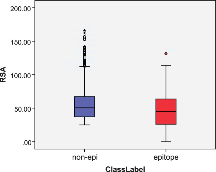
Box plot of RSA for epitopes and non-epitopes

3.3.2 B factor

Another important feature is B factor, which is a characteristic used to indicate the mobility of atoms. The atoms buried in proteins are typically less mobilizable and have a smaller B factor, while those exposed on the surface are more flexible and have a larger B factor. B factor is widely used in studies on protein binding (Chung et al., 2006; Liu et al., 2013; Neuvirth et al., 2004). However, this is the first time B factor has been used as a feature in epitope prediction.

As can be seen from Figure 4a and Table 4, B factor is a notable feature in distinguishing epitope residues from non-epitope residues. The P-value of the Mann–Whitney U hypothesis test on B factor is 0, implying that there are different distributions between epitope residues and non-epitope residues in terms of B factor; in other words, B factor is an effective feature in epitope prediction. In addition, the smoothed B factor along the sequence and the B factor of the nearby residues in the structure window also affect the prediction significantly. A test on the sequence smoothed B factor returns a P-value of 0, which confirms that it is reasonable to use the sequence window in constructing new features.

Figure 6 shows a box-plot of the B factor distribution of epitope residues and non-epitope residues. The average B factor of epitope residues is 39.7, while that of non-epitope residues is 52.27: epitope residues are apt to locate in less mobilizable areas compared with other surface residues.

Fig. 6.

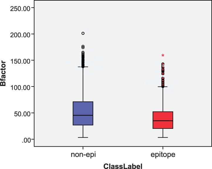
Box plot of B factor distribution for epitopes and non-epitopes

Figure 7 provides an example to illustrate the association of the epitopes with the B factor distribution on A/Hong Kong/1/1968 (H3N2) influenza virus (4FNK). It can be seen that epitopes are mainly located at those residues whose B factor is small. For this example, the epitopes on the stem region (often conserved epitopes) locate at those residues where the B factor is low (blue), while the epitope on the head region (often less conserved) has slightly higher B factors (green). This is because the HA1 itself is more flexible than HA2 and thus has higher B factors.

Fig. 7.

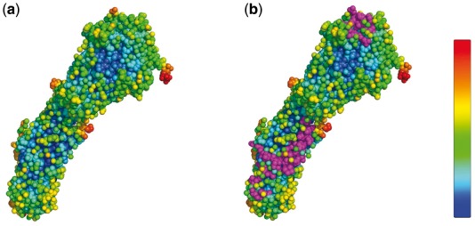
Mapping of B factors with epitope residues on A/Hong Kong/1/1968 (H3N2) influenza virus (4FNK). (a) B factor distribution on 4FNK: the color pattern is shown in the color bar: the color from blue to red represents the B factor from small to large. (b) Epitopes on 4FNK: the epitopes are marked in magenta

3.3.3 Protrusion index

PI, a widely used structural feature (Ponomarenko et al., 2008; Thornton et al., 1986), proves to be effective in the prediction, as shown in Figure 8. The mean PI of epitope residues is 0.87 and that of non-epitope residues is 1.07. That is, epitopes are more concave on the surface. The P-value of the Mann–Whitney U hypothesis test on PI is 0, indicating its effectiveness in identifying epitope residues.

Fig. 8.

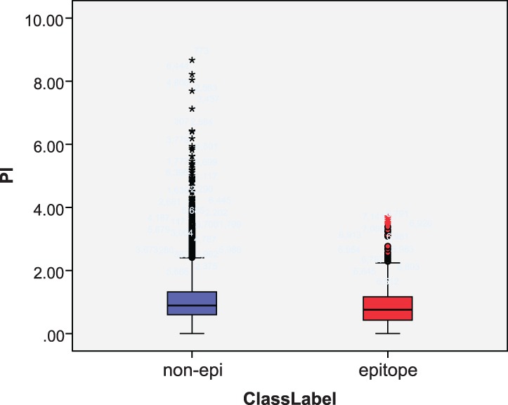
Box plot of PI for epitopes and non-epitopes

3.3.4 Other features

Besides the structural features discussed above, traditional physicochemical features such as β-turns, hydrophobicity and flexibility are also highly ranked in epitope prediction. The epitope residue predictions are affected by physicochemical features of residues that are nearby in sequence or have spatial proximity. As can be seen from Table 4, the top-ranked physicochemical features are mostly smoothed over the sequence window (‘Smoothed’) or the structural window (‘Average’, ‘Maximum’ or ‘Minimum’). In particular, some of them, such as β-turns and hydrophilicity smoothed over the sequence window or the structural window, strongly reflect the influence of nearby residues on epitope residue predictions. Therefore, applying the sequence window and the structure window on these features contributes to the identification of the epitope residues.

4 CASE STUDIES

CeePre is trained on our entire balanced dataset and then applied to the tertiary structure data of an antigen of HIV and an antigen of an influenza virus to make prediction of their epitopes. These two antigens are distantly related to the antigens in our training dataset.

4.1 Antigen GP120 of HIV-1 clade A/E 93TH057

The tertiary structure data of the antigen GP120 of HIV-1 clade A/E 93TH057 is stored at PDB entry 3TGT. There are six complexes (3SE8, 3SE9, 4LSP, 4LSU, 3NGB and 4JB9) containing this antigen or a mutated one in PDB. From these six complexes, we extracted six epitopes for GP120. These epitopes, not all identical, are aggregative and overlapping (Supplementary Fig. S2).

In our training dataset, the only antigen related to HIV virus is an HIV-1 capsid protein (2PXR). Its epitope is extracted from 1AFV (an HIV-1 capsid protein in complex with Fab25.3). But no significant sequence similarity is found between 2PXR and 3TGT (the test antigen GP120) by BLAST. In the training dataset of DiscoTope and SEPPA, however, there are antigens similar to antigen GP120. In fact, DiscoTope’s training data contains 1RZK, 1G9M, 1G9N and 1GC1, which are four envelope glycoprotein GP120 and antibody complexes. In SEPPA, 2I5Y, 1G9M and 1G9N are three envelope glycoprotein GP120 and antibody complexes. Therefore, the comparison is not favorable to CeePre, as the performance of DiscoTope and SEPPA on 3TGT may be overestimated. ElliPro does not need to be trained, and thus it has no training dataset.

4.1.1 Prediction performance comparison

The prediction results of CeePre and those of the other three predictors are reported in Table 5. CeePre achieves good prediction results, outperforming DiscoTope and SEPPA. ElliPro has a slightly higher recall (0.66 versus our 0.61), that is, 66% of the true epitope residues are correctly predicted. However, its precision is only 0.22, meaning that of the residues predicted as epitope residues, only 22% are true epitope residues. In other words, it tends to predict non-epitope residues as epitope residues. As to CeePre2, although the recall value is slightly less than ElliPro (0.05 lower), its accuracy is significantly higher (0.51 higher). Thus, it achieves an F-score of 0.55, which is twice as high as that of ElliPro. Also, our MCC is much better (0.58 versus −0.08). The comparison result can be seen more clearly in Figure 9c and e.

Table 5.

Prediction performance on the HIV antigen GP120 (3TGT)

Methods	F-score	Precision	Recall	MCC	Specificity	Accuracy
CeePre1	0.59	0.61	0.57	0.47	0.89	0.81
CeePre2	0.67	0.73	0.61	0.58	0.93	0.85
DiscoTope	0.55	0.55	0.55	0.40	0.86	0.78
ElliPro	0.33	0.22	0.66	−0.08	0.26	0.35
SEPPA	0.38	0.31	0.50	0.13	0.65	0.62

Fig. 9.

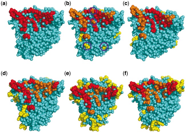
Epitope prediction for antigen GP120 of an HIV virus. (a) The true epitope residues. (b) and (c) Prediction results by our methods CeePre1 and CeePre2 respectively. (d–f) Prediction results by other methods DiscoTope, ElliPro and SEPPA respectively. TP predictions are in red, FN predictions are in orange, FP predictions are in yellow and the background cyan represents TN predictions. The purple circles in sub-figure (b) mark those residues that are wrongly predicted as an isolated epitope or a non-epitope residue by CeePre1 and are corrected by clustering in CeePre2

4.1.2 The clustering effect of the new features used by CeePre2

As can be seen from Figure 9a–c, 61% of the true epitope residues are identified by CeePre2. Compared with CeePre1, CeePre2 has an impressive clustering effect on true epitope residues. Some non-epitope residue predictions among true epitope residue predictions are also corrected as true epitope residues by CeePre2. At the same time, CeePre2 corrects predictions for some isolated residues that are all predicted as antigenic residue by CeePre 1, for example, residues at positions 47, 53, 57, 63, 68, 232, 234, 236, 247, 250, 299, 439 and 444 in chain A, which are all false-positive predictions by CeePre1.

4.2 Antigen hemagglutinin of influenza A/Japan/305/1957(H2N2)

Our prediction models CeePre1 and CeePre2 are also applied to the tertiary structure data (3KU3) of antigen hemagglutinin (HA) of an influenza virus A/Japan/305/1957(H2N2). This antigen has two quaternary structures in PDB: 4HF5 (A/Japan/305/1957 in complex with Fab 8F8) and 4HLZ (A/Japan/305/1957 in complex with a broadly neutralizing antibody C179 (Dreyfus et al., 2013).

In our training dataset, only one tertiary structure (2YPG) is from the influenza family, and its three epitopes (extracted from 1EO8, 1QFU, 1KEN) are all annotated. The evolution distance between the two antigens is far: 3KU3 HA belongs to group 1, while 2YPG HA belongs to group 2. Their sequence similarity determined by BLAST is only 36% for HA1 and 56% for HA2. HA in group 1 is not included in the training datasets of DiscoTope, ElliPro or SEPPA either. Thus, this is a fair comparison.

4.2.1 Prediction performance comparison on 3KU3

The prediction results are listed in Table 6. The performance by CeePre2 excels for every metric compared with the three predictors. Its F-score is more than twice of the best of the other three predictors. For MCC, another metric that characterizes the overall performance of classifiers, CeePre2 far exceeds all three predictors. There is a remarkable improvement in recall, which implies that more epitope residues are identified by CeePre2. At the same time, the precision and specificity of CeePre2 are also higher.

Table 6.

Test performance on influenza virus antigen HA (3KU3)

Methods	F-score	Precision	Recall	MCC	Specificity	Accuracy
CeePre1	0.49	0.37	0.71	0.41	0.82	0.80
CeePre2	0.43	0.29	0.83	0.36	0.69	0.70
DiscoTope	0.19	0.13	0.37	−0.01	0.62	0.58
ElliPro	0.21	0.12	0.60	−0.03	0.35	0.39
SEPPA	0.21	0.14	0.37	0.02	0.66	0.62

Compared with CeePre1, CeePre2 makes a significant improvement on recall, but shows a relatively small decrease in specificity and precision. This means that more true epitope residues are correctly classified, but some non-epitope residues are marked as epitope residues. Next, we will discuss the reason for this phenomenon.

4.2.2 Some prediction details

Figure 10 shows that the two epitopes of the HA are correctly identified by CeePre. All the antigenic residues of the epitope binding to 8F8 are correctly predicted by CeePre2. This epitope is on HA1. Almost all of the antigenic residues of the epitope on HA2 that binds to the broadly neutralizing antibody C179 are correctly predicted. A small number of edge antigenic residues (residues 38, 40, 291 on chain A and residues 42, 45, 56 on chain B) are predicted as negative. This may be because this epitope is conserved; it has a slightly different feature from strain-specific epitopes and may need special strategies for epitope prediction and feature selection. As can be seen in Figure 10d–f, this conserved epitope is not detected by the other three predictors.

Fig. 10.

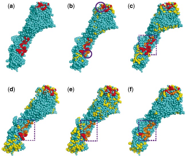
Epitope prediction for antigen HA of an influenza virus (3KU3). (a) The true epitope residues. (b) and (c) Prediction results by our methods CeePre1 and CeePre2 respectively. (d–f) Prediction results by other methods DiscoTope, ElliPro and SEPPA respectively. The colors and the purple circles have the same meaning as those in Figure 9. The purple dashed box in sub-figures (c–f) marks the position of the conserved epitope on HA2

CeePre2 again demonstrates the clustering effect on this antigen: separated antigenic residues are aggregated into epitopes, while isolated epitope and non-epitope residue predictions by CeePre1 are removed by the second stage of CeePre2. The precision and specificity may decrease in this stage, especially for those antigens whose epitopes are not completely discovered or annotated (high FP). For example, although some antibodies have been proved to react with the virus A/Japan/305/1957(H2N2), for example, C05 and CR6261 (Ekiert et al., 2012), their complex structures are not yet determined and the epitopes are still unknown. These epitope residues cannot be annotated here, leading to a higher FP rate.

5 CONCLUSION

In this article, we have proposed CeePre for conformational B-cell epitope prediction. CeePre has a two-stage learning strategy for the random forest algorithm to identify clusters of antigenic residues. It incorporates various basic features as well as extended composite features through a sequence window and a structure window. Of these features, B factor is used for the first time for B-cell epitope prediction It has been found to be effective in epitope prediction.

To be practically useful, a tertiary structure dataset has been constructed for the training of our prediction method and has also been used in the evaluation of CeePre. Compared with three widely used structure-based epitope prediction models, our CeePre shows a significant improvement in prediction performance.

For deep case studies, CeePre has been applied to the epitope prediction for two antigens that are distantly related to our training data. One antigen is an HIV antigen, the other is an influenza antigen. It has been found that CeePre not only obtains more accurate predictions of epitope residues but also forms more meaningful epitope predictions by clustering adjacent residues.

Funding: This research work was supported by a UTS 2013 Early Career Research Grant; an ARC Discovery Project (DP130102124); and the China Scholarship Council (J.R.).

Conflict of Interest: none declared.

REFERENCES

- Andersen PH, et al. Prediction of residues in discontinuous B-cell epitopes using protein 3d structures. Protein Sci. 2006;15:2558–2567. doi: 10.1110/ps.062405906. [DOI] [PMC free article] [PubMed] [Google Scholar]
- Blythe MJ, Flower DR. Benchmarking B cell epitope prediction: underperformance of existing methods. Protein Sci. 2005;14:246–248. doi: 10.1110/ps.041059505. [DOI] [PMC free article] [PubMed] [Google Scholar]
- Breiman L. Random forests. Mach. Learn. 2001;45:5–32. [Google Scholar]
- Chen J, et al. Prediction of linear B-cell epitopes using amino acid pair antigenicity scale. Amino Acids. 2007;33:423–428. doi: 10.1007/s00726-006-0485-9. [DOI] [PubMed] [Google Scholar]
- Chou PY, Fasman GD. Conformational parameters for amino acids in helical, β-sheet, and random coil regions calculated from proteins. Biochemistry. 1974;13:211–222. doi: 10.1021/bi00699a001. [DOI] [PubMed] [Google Scholar]
- Chung J, et al. Exploiting sequence and structure homologs to identify protein-protein binding sites. Proteins. 2006;62:630–640. doi: 10.1002/prot.20741. [DOI] [PubMed] [Google Scholar]
- Deng L, et al. Prediction of protein-protein interaction sites using an ensemble method. BMC Bioinformatics. 2009;10:426. doi: 10.1186/1471-2105-10-426. [DOI] [PMC free article] [PubMed] [Google Scholar]
- Dreyfus C, et al. Structure of a classical broadly neutralizing stem antibody in complex with a pandemic h2 influenza virus hemagglutinin. J. Virol. 2013;87:7149–7154. doi: 10.1128/JVI.02975-12. [DOI] [PMC free article] [PubMed] [Google Scholar]
- Ekiert DC, et al. Cross-neutralization of influenza a viruses mediated by a single antibody loop. Nature. 2012;489:526–532. doi: 10.1038/nature11414. [DOI] [PMC free article] [PubMed] [Google Scholar]
- El-Manzalawy Y, et al. BIBM’08: IEEE International Conference on Bioinformatics and Biomedicine. 2008. Predicting protective linear B-cell epitopes using evolutionary information; pp. 289–292. [Google Scholar]
- Han J, et al. Data Mining: Concepts and Techniques. San Francisco, USA: Morgan Kaufmann; 2006. [Google Scholar]
- Hopp TP, Woods KR. Prediction of protein antigenic determinants from amino acid sequences. Proc. Natl Acad. Sci. USA. 1981;78:3824–3828. doi: 10.1073/pnas.78.6.3824. [DOI] [PMC free article] [PubMed] [Google Scholar]
- Janin J. Surface and inside volumes in globular proteins. Nature. 1979;277:491–492. doi: 10.1038/277491a0. [DOI] [PubMed] [Google Scholar]
- Jordan R. 2010. A structural-based two-stage classifier for predicting protein-protein interface residues. Technical Report, Iowa State University. [Google Scholar]
- Karplus P, Schulz G. Prediction of chain flexibility in proteins. Naturwissenschaften. 1985;72:212–213. [Google Scholar]
- Kawashima S, et al. AAIndex: amino acid index database, progress report 2008. Nucleic Acids Res. 2008;36(Suppl. 1):D202–D205. doi: 10.1093/nar/gkm998. [DOI] [PMC free article] [PubMed] [Google Scholar]
- Kolaskar A, Tongaonkar PC. A semi-empirical method for prediction of antigenic determinants on protein antigens. FEBS Lett. 1990;276:172–174. doi: 10.1016/0014-5793(90)80535-q. [DOI] [PubMed] [Google Scholar]
- Kringelum JV, et al. Structural analysis of B-cell epitopes in antibody: protein complexes. Mol. Immunol. 2013;53:24–34. doi: 10.1016/j.molimm.2012.06.001. [DOI] [PMC free article] [PubMed] [Google Scholar]
- Kulkarni-Kale U, et al. CEP: a conformational epitope prediction server. Nucleic Acids Res. 2005;33(Suppl. 2):W168–W171. doi: 10.1093/nar/gki460. [DOI] [PMC free article] [PubMed] [Google Scholar]
- Larsen JE, et al. Improved method for predicting linear B-cell epitopes. Immunome Res. 2006;2:2. doi: 10.1186/1745-7580-2-2. [DOI] [PMC free article] [PubMed] [Google Scholar]
- Liaw A, Wiener M. Classification and regression by randomForest. R News. 2002;2:18–22. [Google Scholar]
- Liu Q, et al. Binding affinity prediction for protein-ligand complexes based on beta contacts and B factor. J. Chem. Inf. Model. 2013;53:3076–3085. doi: 10.1021/ci400450h. [DOI] [PubMed] [Google Scholar]
- Lo YT, et al. Prediction of conformational epitopes with the use of a knowledge-based energy function and geometrically related neighboring residue characteristics. BMC Bioinformatics. 2013;14(Suppl. 4):S3. doi: 10.1186/1471-2105-14-S4-S3. [DOI] [PMC free article] [PubMed] [Google Scholar]
- Mihel J, et al. PSAIA-protein structure and interaction analyzer. BMC Struct. Biol. 2008;8:21. doi: 10.1186/1472-6807-8-21. [DOI] [PMC free article] [PubMed] [Google Scholar]
- Moreau V, et al. PEPOP: computational design of immunogenic peptides. BMC Bioinformatics. 2008;9:71. doi: 10.1186/1471-2105-9-71. [DOI] [PMC free article] [PubMed] [Google Scholar]
- Neuvirth H, et al. ProMate: a structure based prediction program to identify the location of proteinprotein binding sites. J. Mol. Biol. 2004;338:181–199. doi: 10.1016/j.jmb.2004.02.040. [DOI] [PubMed] [Google Scholar]
- Parker J, et al. New hydrophilicity scale derived from high-performance liquid chromatography peptide retention data: correlation of predicted surface residues with antigenicity and X-ray-derived accessible sites. Biochemistry. 1986;25:5425–5432. doi: 10.1021/bi00367a013. [DOI] [PubMed] [Google Scholar]
- Pellequer JL, et al. Correlation between the location of antigenic sites and the prediction of turns in proteins. Immunology Lett. 1993;36:83–99. doi: 10.1016/0165-2478(93)90072-a. [DOI] [PubMed] [Google Scholar]
- Ponomarenko JV, Bourne PE. Antibody-protein interactions: benchmark datasets and prediction tools evaluation. BMC Struct. Biol. 2007;7:64. doi: 10.1186/1472-6807-7-64. [DOI] [PMC free article] [PubMed] [Google Scholar]
- Ponomarenko J, et al. ElliPro: a new structure-based tool for the prediction of antibody epitopes. BMC Bioinformatics. 2008;9:514. doi: 10.1186/1471-2105-9-514. [DOI] [PMC free article] [PubMed] [Google Scholar]
- Rost B, Sander C. Conservation and prediction of solvent accessibility in protein families. Proteins. 1994;20:216–226. doi: 10.1002/prot.340200303. [DOI] [PubMed] [Google Scholar]
- Saha S, Raghava G. Prediction of continuous B-cell epitopes in an antigen using recurrent neural network. Proteins. 2006;65:40–48. doi: 10.1002/prot.21078. [DOI] [PubMed] [Google Scholar]
- Sollner J, et al. Analysis and prediction of protective continuous B-cell epitopes on pathogen proteins. Immunome Res. 2008;4:1. doi: 10.1186/1745-7580-4-1. [DOI] [PMC free article] [PubMed] [Google Scholar]
- Sun J, et al. SEPPA: a computational server for spatial epitope prediction of protein antigens. Nucleic Acids Res. 2009;37(Suppl. 2):W612–W616. doi: 10.1093/nar/gkp417. [DOI] [PMC free article] [PubMed] [Google Scholar]
- Swapna LS, et al. Roles of residues in the interface of transient protein-protein complexes before complexation. Sci. Rep. 2012;2:334. doi: 10.1038/srep00334. [DOI] [PMC free article] [PubMed] [Google Scholar]
- Sweredoski MJ, Baldi P. PEPITO: improved discontinuous B-cell epitope prediction using multiple distance thresholds and half sphere exposure. Bioinformatics. 2008;24:1459–1460. doi: 10.1093/bioinformatics/btn199. [DOI] [PubMed] [Google Scholar]
- Thornton J, et al. Location of’continuous’ antigenic determinants in the protruding regions of proteins. EMBO J. 1986;5:409. doi: 10.1002/j.1460-2075.1986.tb04226.x. [DOI] [PMC free article] [PubMed] [Google Scholar]
- Westhof E. PREDITOP: a program for antigenicity prediction. J. Mol. Graph. 1993;11:204–210. doi: 10.1016/0263-7855(93)80074-2. [DOI] [PubMed] [Google Scholar]
- Zhao L, et al. Antibody-specified B-cell epitope prediction in line with the principle of context-awareness. IEEE/ACM Trans. Comput. Biol. Bioinform. 2011;8:1483–1494. doi: 10.1109/TCBB.2011.49. [DOI] [PubMed] [Google Scholar]
- Zhao L, et al. B-cell epitope prediction through a graph model. BMC Bioinformatics. 2012;13(Suppl. 17):S20. doi: 10.1186/1471-2105-13-S17-S20. [DOI] [PMC free article] [PubMed] [Google Scholar]