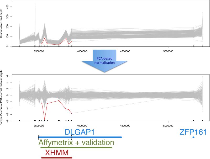
Figure 10. XHMM copy number variation region plot.

This plot shows each sample's original and normalized read depths at each of the targets in focus, which are connected by gray lines. If the sample has a called deletion, then it is colored in red, and duplications in green. Gene names are added below to annotate the genomic region, and black dots and bars mark the location of the exome targets. In this example from the XHMM paper (Fromer et al. 2012), also shown are the overlaps between the XHMM call (marked in red), the Affymetrix chip-based call and custom validated region (Kirov et al. 2012), and the exome-targeted region of DLGAP1 (delineated by square brackets). By following Basic Protocol 2, a regional plot is produced for each CNV called in each individual (as found in the .xcnv file): plot_CNV/sample_*.png. Alternatively, a PDF with all stages of read depth adjustment (from unnormalized [top panel here] to final normalized values used for CNV calling [bottom panel here]) can be generated by passing the PLOT_ONLY_PNG=FALSE argument to the XHMM_plots() function in the example_make_XHMM_plots.R script file.