Figure - PMC

Skip to main content

An official website of the United States government

Here's how you know

Here's how you know

Official websites use .gov
A .gov website belongs to an official government organization in the United States.

Secure .gov websites use HTTPS
A lock ( ) or https:// means you've safely connected to the .gov website. Share sensitive information only on official, secure websites.

View full-text article in PMC

. 2014 Apr 25;42(11):e94. doi: 10.1093/nar/gku343

Search in PMC
Search in PubMed
View in NLM Catalog
Add to search

© The Author(s) 2014. Published by Oxford University Press on behalf of Nucleic Acids Research.

This is an Open Access article distributed under the terms of the Creative Commons Attribution License (http://creativecommons.org/licenses/by/3.0/), which permits unrestricted reuse, distribution, and reproduction in any medium, provided the original work is properly cited.

PMC Copyright notice

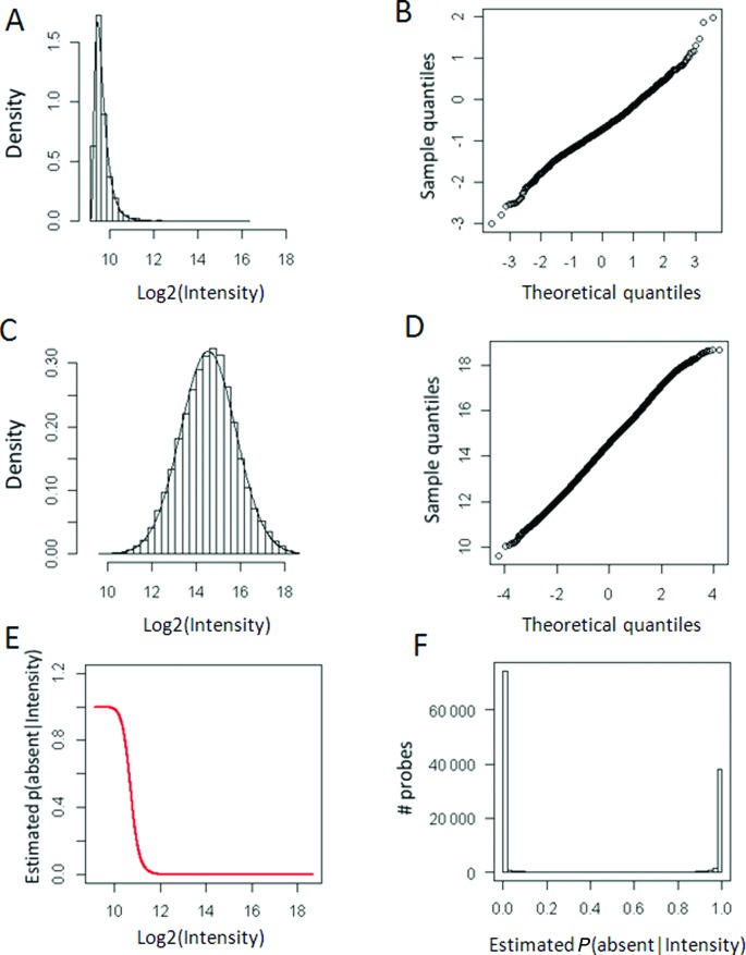
Figure 3. — Goodness of fit and outcome of the empirical statistical modeling procedure. (A) Histogram and density plot showing the fit of the shifted log-normal distribution to the intensities of the negative-control probes. (B) Quantile–quantile plot showing the fit of the shifted log-normal distribution to the intensities of the negative-control probes. (C) Histogram and density plot showing the fit of the normal distribution to the intensities of the perfect-match probes. (D) Quantile-quantile plot showing the fit of the normal distribution to the intensities of the perfect-match probes. (E) Bayesian P-values plotted against probe-signal intensity. (F) Histogram showing the distribution of the P(absent|intensity) values.